Bayes Theorem Basics Total probability Theorem Bayes Theorem
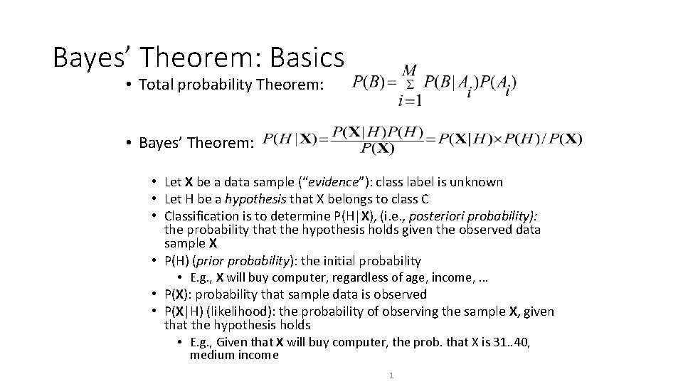
Bayes’ Theorem: Basics • Total probability Theorem: • Bayes’ Theorem: • Let X be a data sample (“evidence”): class label is unknown • Let H be a hypothesis that X belongs to class C • Classification is to determine P(H|X), (i. e. , posteriori probability): the probability that the hypothesis holds given the observed data sample X • P(H) (prior probability): the initial probability • E. g. , X will buy computer, regardless of age, income, … • P(X): probability that sample data is observed • P(X|H) (likelihood): the probability of observing the sample X, given that the hypothesis holds • E. g. , Given that X will buy computer, the prob. that X is 31. . 40, medium income 1
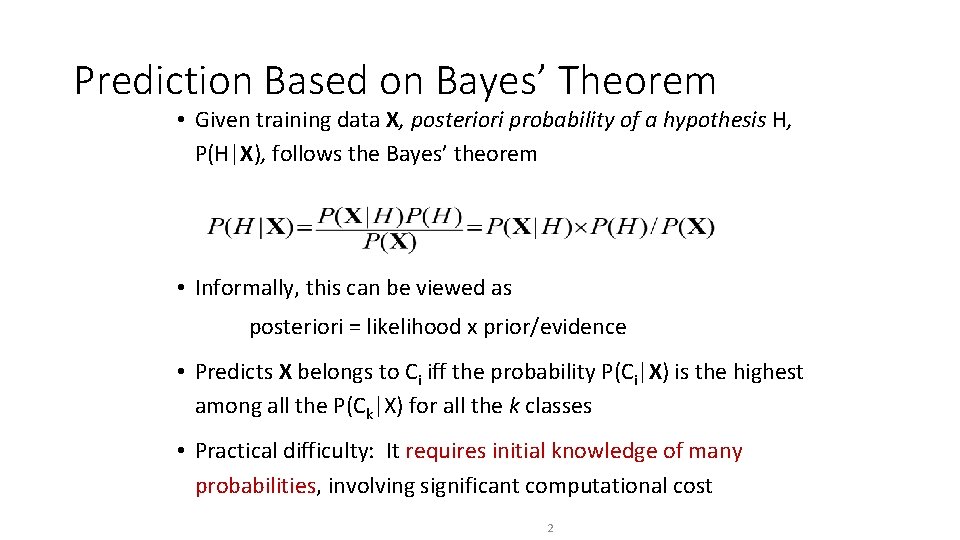
Prediction Based on Bayes’ Theorem • Given training data X, posteriori probability of a hypothesis H, P(H|X), follows the Bayes’ theorem • Informally, this can be viewed as posteriori = likelihood x prior/evidence • Predicts X belongs to Ci iff the probability P(Ci|X) is the highest among all the P(Ck|X) for all the k classes • Practical difficulty: It requires initial knowledge of many probabilities, involving significant computational cost 2

Classification is to Derive the Maximum Posteriori • Let D be a training set of tuples and their associated class labels, and each tuple is represented by an n-D attribute vector X = (x 1, x 2, …, xn) • Suppose there are m classes C 1, C 2, …, Cm. • Classification is to derive the maximum posteriori, i. e. , the maximal P(Ci|X) • This can be derived from Bayes’ theorem • Since P(X) is constant for all classes, only needs to be maximized 3
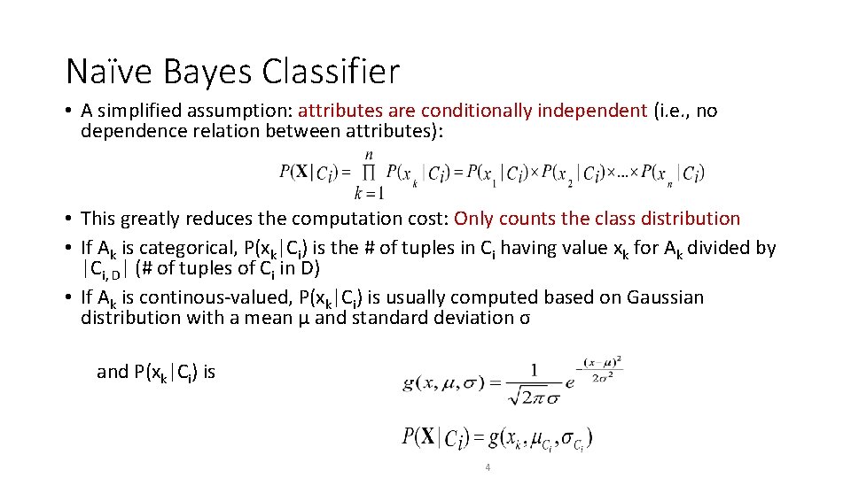
Naïve Bayes Classifier • A simplified assumption: attributes are conditionally independent (i. e. , no dependence relation between attributes): • This greatly reduces the computation cost: Only counts the class distribution • If Ak is categorical, P(xk|Ci) is the # of tuples in Ci having value xk for Ak divided by |Ci, D| (# of tuples of Ci in D) • If Ak is continous-valued, P(xk|Ci) is usually computed based on Gaussian distribution with a mean μ and standard deviation σ and P(xk|Ci) is 4
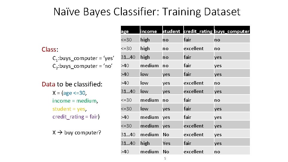
Naïve Bayes Classifier: Training Dataset Class: C 1: buys_computer = ‘yes’ C 2: buys_computer = ‘no’ Data to be classified: X = (age <=30, income = medium, student = yes, credit_rating = fair) X buy computer? age income student credit_rating buys_computer <=30 high no fair no <=30 high no excellent no 31… 40 high no fair yes >40 medium no fair yes >40 low yes excellent no 31… 40 low yes excellent yes <=30 medium no fair no <=30 low yes fair yes >40 medium yes fair yes <=30 medium yes excellent yes 31… 40 medium No excellent yes 31… 40 high fair yes excellent no >40 Yes medium No 5
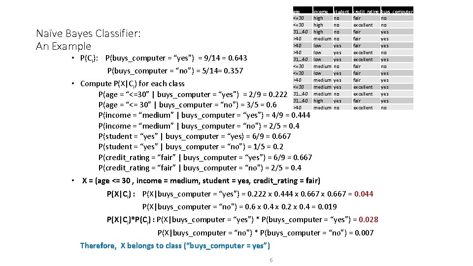
Naïve Bayes Classifier: An Example • P(Ci): P(buys_computer = “yes”) = 9/14 = 0. 643 P(buys_computer = “no”) = 5/14= 0. 357 age income student credit_rating buys_computer <=30 31… 40 >40 >40 31… 40 <=30 >40 <=30 31… 40 >40 high medium low low medium high medium no no yes yes yes no • Compute P(X|Ci) for each class P(age = “<=30” | buys_computer = “yes”) = 2/9 = 0. 222 P(age = “<= 30” | buys_computer = “no”) = 3/5 = 0. 6 P(income = “medium” | buys_computer = “yes”) = 4/9 = 0. 444 P(income = “medium” | buys_computer = “no”) = 2/5 = 0. 4 P(student = “yes” | buys_computer = “yes) = 6/9 = 0. 667 P(student = “yes” | buys_computer = “no”) = 1/5 = 0. 2 P(credit_rating = “fair” | buys_computer = “yes”) = 6/9 = 0. 667 P(credit_rating = “fair” | buys_computer = “no”) = 2/5 = 0. 4 fair excellent fair fair excellent fair excellent • X = (age <= 30 , income = medium, student = yes, credit_rating = fair) P(X|Ci) : P(X|buys_computer = “yes”) = 0. 222 x 0. 444 x 0. 667 = 0. 044 P(X|buys_computer = “no”) = 0. 6 x 0. 4 x 0. 2 x 0. 4 = 0. 019 P(X|Ci)*P(Ci) : P(X|buys_computer = “yes”) * P(buys_computer = “yes”) = 0. 028 P(X|buys_computer = “no”) * P(buys_computer = “no”) = 0. 007 Therefore, X belongs to class (“buys_computer = yes”) 6 no no yes yes yes no
Tahapan Algoritma Naïve Bayes 1. 2. 3. 4. Baca Data Training Hitung jumlah class Hitung jumlah kasus yang sama dengan class yang sama Kalikan semua nilai hasil sesuai dengan data X yang dicari class-nya 7

1. Baca Data Training 8

Teorema Bayes • X • H • • Data dengan class yang belum diketahui Hipotesis data X yang merupakan suatu class yang lebih spesifik P (H|X) Probabilitas hipotesis H berdasarkan kondisi X (posteriori probability) P (H) Probabilitas hipotesis H (prior probability) P (X|H) Probabilitas X berdasarkan kondisi pada hipotesis H P (X) Probabilitas X 9
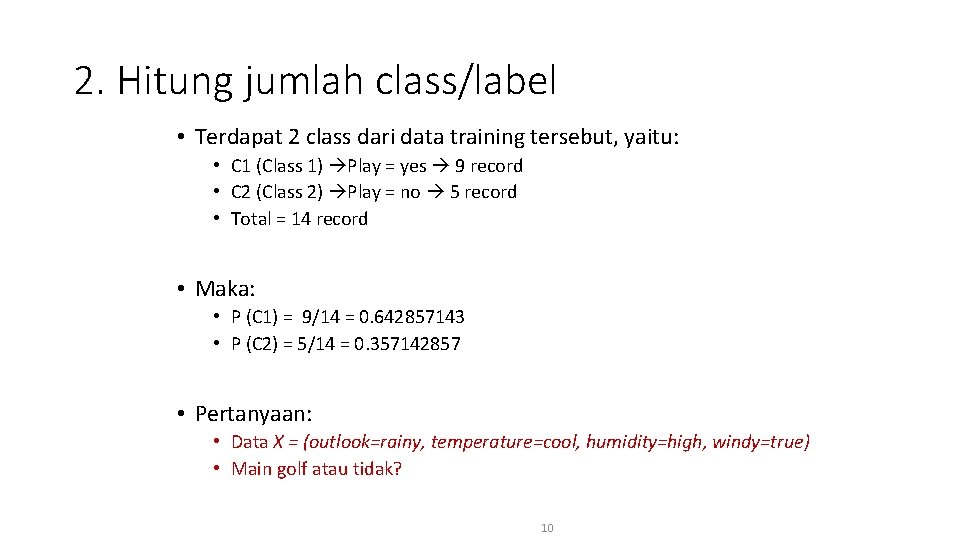
2. Hitung jumlah class/label • Terdapat 2 class dari data training tersebut, yaitu: • C 1 (Class 1) Play = yes 9 record • C 2 (Class 2) Play = no 5 record • Total = 14 record • Maka: • P (C 1) = 9/14 = 0. 642857143 • P (C 2) = 5/14 = 0. 357142857 • Pertanyaan: • Data X = (outlook=rainy, temperature=cool, humidity=high, windy=true) • Main golf atau tidak? 10

3. Hitung jumlah kasus yang sama dengan class yang sama • Untuk P(Ci) yaitu P(C 1) dan P(C 2) sudah diketahui hasilnya di langkah sebelumnya. • Selanjutnya Hitung P(X|Ci) untuk i = 1 dan 2 • P(outlook=“sunny”|play=“yes”)=2/9=0. 22222 • P(outlook=“sunny”|play=“no”)=3/5=0. 6 • P(outlook=“overcast”|play=“yes”)=4/9=0. 44444 • P(outlook=“overcast”|play=“no”)=0/5=0 • P(outlook=“rainy”|play=“yes”)=3/9=0. 33333 • P(outlook=“rainy”|play=“no”)=2/5=0. 4 11
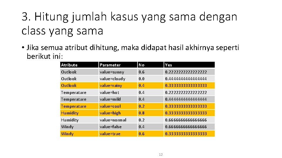
3. Hitung jumlah kasus yang sama dengan class yang sama • Jika semua atribut dihitung, maka didapat hasil akhirnya seperti berikut ini: Atribute Outlook Temperature Humidity Windy Parameter value=sunny value=cloudy value=rainy value=hot value=mild value=cool value=high value=normal value=false value=true No 0. 6 0. 0 0. 4 0. 2 0. 8 0. 2 0. 4 0. 6 Yes 0. 2222222222222222 0. 4444444444444444 0. 3333333333333333 0. 6666666666666666 0. 33333333 12

4. Kalikan semua nilai hasil sesuai dengan data X yang dicari class-nya • Pertanyaan: • Data X = (outlook=rainy, temperature=cool, humidity=high, windy=true) • Main Golf atau tidak? • Kalikan semua nilai hasil dari data X • P(X|play=“yes”) = 0. 333333333* 0. 33333*0. 33333 = 0. 012345679 • P(X|play=“no”) = 0. 4*0. 2*0. 8*0. 6=0. 0384 • P(X|play=“yes”)*P(C 1) = 0. 012345679*0. 642857143 = 0. 007936508 • P(X|play=“no”)*P(C 2) = 0. 0384*0. 357142857 = 0. 013714286 • Nilai “no” lebih besar dari nilai “yes” maka class dari data X tersebut adalah “No” 13

Avoiding the Zero-Probability Problem • Naïve Bayesian prediction requires each conditional prob. be non-zero. Otherwise, the predicted prob. will be zero • Ex. Suppose a dataset with 1000 tuples, income=low (0), income= medium (990), and income = high (10) • Use Laplacian correction (or Laplacian estimator) • Adding 1 to each case Prob(income = low) = 1/1003 Prob(income = medium) = 991/1003 Prob(income = high) = 11/1003 • The “corrected” prob. estimates are close to their “uncorrected” counterparts 14
Naïve Bayes Classifier: Comments • Advantages • Easy to implement • Good results obtained in most of the cases • Disadvantages • Assumption: class conditional independence, therefore loss of accuracy • Practically, dependencies exist among variables, e. g. : • Hospitals Patients Profile: age, family history, etc. • Symptoms: fever, cough etc. , • Disease: lung cancer, diabetes, etc. • Dependencies among these cannot be modeled by Naïve Bayes Classifier • How to deal with these dependencies? Bayesian Belief Networks 15
- Slides: 15