Bayes for Beginners STEPHANIE AZZOPARDI HRVOJE STOJIC SUPERVISOR

Bayes for Beginners STEPHANIE AZZOPARDI & HRVOJE STOJIC SUPERVISOR: DR PETER ZEIDMAN 7 T H DECEMBER 2016

What is Bayes? Frequentist statistics – p values and confidence intervals Bayesian statistics deal with conditional variability. Apply variable parameters to fixed data – update our beliefs based on new knowledge Wide range of applications

Probability of A occurring: P(A) Probability of B occurring: P(B) Joint probability (A AND B both occurring): P(A, B)

Marginal Probability Diabetes No Diabetes Neuropathy 0. 3 0. 1 No neuropathy 0. 1 0. 5

Marginal Probability What are the chances of a patient having neuropathy? P(neuropathy) = 0. 4 P(neuropathy) = ∑ P(neuropathy , diabetes) diabetes Joint Probability P(A) = ∑ P(A , B) P(diabetes, neuropathy) = 0. 5 B

Conditional probability What is the probability of a patient having neuropathy, given that he has diabetes? Probability of A given B?

Conditional Probability This also works in reverse, i. e. P(A, B) Joint probability can be expressed as: P(A) P(A, B) = P(A|B)*P(B) P(A, B) = P(B|A)*P(A)

Bayes’s equation Likelihood Posterior Denominator Prior

Example 1

Example 2 A disease occurs in 0. 5% of population A diagnostic test gives a positive result in: ◦ 99% of people with the disease ◦ 5% of people without the disease (false positive) A person receives a positive result. What is the probability of them having the disease, given a positive result?

P(disease|positive test result) = P(positive test/disease) x P (disease) P(positive test) We know: P(positive test/disease) = 0. 99 P(disease) = 0. 005 P(positive test) = ? ? ?

P(B) = P(B|A) * P(A) + P(B|~A) * P(~A) = (0. 99 * 0. 005) + (0. 05 * 0. 995) = 0. 055 Where: P(A) = chance of disease P(~A) = chance of not having the disease. Remember: P (~A) = 1 – P(A) P(B|A) = chance of positive test given that disease is present P(B|~A) = chance of positive test given that the disease isn’t present

Therefore: P(disease/positive test result) = 0. 99 x 0. 005 = 0. 09 i. e. 9% 0. 055

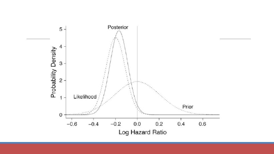
Bayesian Statistics Provides a dynamic model through which our belief is constantly updated as we add more data. Ultimate goal is to calculate the posterior probability density, which is proportional to the likelihood (of our data being correct) and our prior knowledge. Can be used as model for the brain (Bayesian brain), history and human behaviour.

Frequentist vs. Bayesian statistics

Frequentist models in practice l. Model: y = Xθ + ε l l. Data, X, is random variable, while parameters, θ, are fixed. l l. Hence, we assume there is a true set of parameters, or true model of the world, and we are concerned with getting the best possible estimate. l l. We are interested in point estimates of parameters given the data.

Bayesian models in practice l. Model: y = Xθ + ε l l. Data, X, is fixed, while parameters, θ, are considered to be random variables. l l. There is no single set of parameters that denotes a true model of the world - we have parameters that are more or less probable. l l. We are interested in distribution of parameters given the data.

Bayes rule – slightly different form Prior Likelihood Posterior P(θ|X) = P(X|θ) x P(θ) P(X) Marginal 1. How good are our parameters given the data 1. Prior knowledge is incorporated and used to update our beliefs about the parameters

Coin flipping model • Someone flips coin. • We don’t know if the coin is fair or not. • We are told only the outcome of the coin flipping.

Coin flipping model • 1 st Hypothesis: Coin is fair, 50% Heads or Tails • • • 2 nd Hypothesis: Both side of the coin is heads, 100% Heads

Coin flipping model • 1 st Hypothesis: Coin is fair, 50% Heads or Tails P(A = fair coin) = 0. 99 • • 2 nd Hypothesis: Both side of the coin is heads, 100% Heads P(-A = unfair coin) = 0. 01

Coin flipping model •

Coin flipping model •

Coin flipping model •

Coin flipping model Coin is flipped a second time and it is heads again. Posterior in the previous time step becomes the new prior!!

Coin flipping model •

Hypothesis testing Classical • Define the null hypothesis • H 0: Coin is fair θ=0. 5 Bayesian Inference • Define a hypothesis • H: θ>0. 1 • 0. 1

Model Selection

Model Selection Marginal likelihood Bayes Factor

Model Selection

Bayesian Models of Cognition

Multi-modal sensory integration How wide is the pen? The pen is 8 mm wide There is a 95% chance that the pen is between 7. 5 and 8. 49 mm wide Probability density function (PDF) Represents both the average estimate of the quantity itself and the confidence in that estimate precision O’Reilly et al, EJN 2012(35), 1169 -72

Multi-modal sensory integration • Humans do show near-Bayesian behaviour in multi-sensory integration tasks • Non-optimal bias to give more weight to one sensory modality than another VISION PROPRIOCEPTION Van Beers et al, Exp Brain Res 1999; 125: 43 -9

Multi-modal sensory integration P(width|touch, vision) P(touch, vision|width) * P(width) • The posterior estimate is biased towards the prior mean Posterior Observed Prior 5 7 • Prior permits to increase accuracy, useful considering uncertainty of observations Width (mm) O’Reilly et al, EJN 2012(35), 1169 -72

Multi-modal sensory integration The Muller-Lyer Illusion Priors could be acquired trough long experience with the environment Some others priors seem to be innate

References Previous Mf. D slides Bayesian statistics: a comprehensive course – video tutorials https: //www. youtube. com/watch? v=U 1 Hb. B 0 ATZ_A&index=1&list=PLFDb. Gp 5 Yz jq. XQ 4 o. E 4 w 9 GVWdiok. WB 9 g. Epm Bayesian statistics (a very brief introduction) – Ken Rice http: //www. statisticshowto. com/bayes-theorem-problems/