Bayes Classifier A probabilistic framework for solving classification
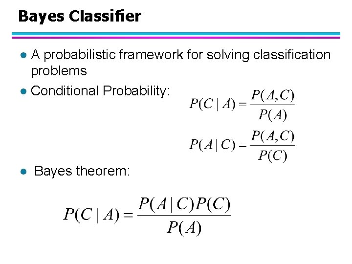
Bayes Classifier A probabilistic framework for solving classification problems l Conditional Probability: l l Bayes theorem:
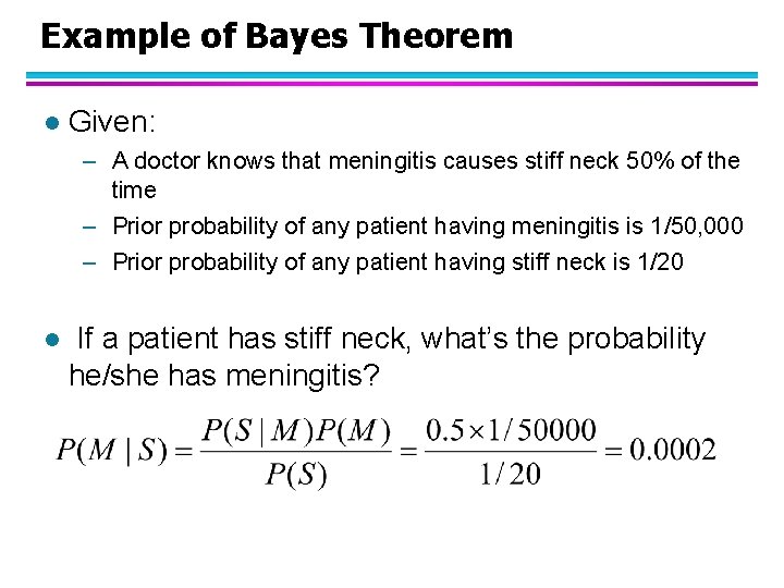
Example of Bayes Theorem l Given: – A doctor knows that meningitis causes stiff neck 50% of the time – Prior probability of any patient having meningitis is 1/50, 000 – Prior probability of any patient having stiff neck is 1/20 l If a patient has stiff neck, what’s the probability he/she has meningitis?
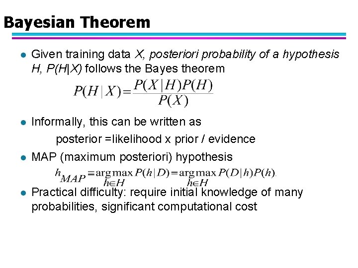
Bayesian Theorem l Given training data X, posteriori probability of a hypothesis H, P(H|X) follows the Bayes theorem l Informally, this can be written as posterior =likelihood x prior / evidence MAP (maximum posteriori) hypothesis l l Practical difficulty: require initial knowledge of many probabilities, significant computational cost
Bayesian Classifiers l Consider each attribute and class label as random variables l Given a record with attributes (A 1, A 2, …, An) – Goal is to predict class C – Specifically, we want to find the value of C that maximizes P(C| A 1, A 2, …, An ) l Can we estimate P(C| A 1, A 2, …, An ) directly from data?
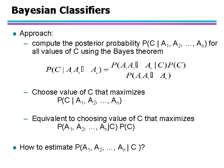
Bayesian Classifiers l Approach: – compute the posterior probability P(C | A 1, A 2, …, An) for all values of C using the Bayes theorem – Choose value of C that maximizes P(C | A 1, A 2, …, An) – Equivalent to choosing value of C that maximizes P(A 1, A 2, …, An|C) P(C) l How to estimate P(A 1, A 2, …, An | C )?
Naïve Bayes Classifier l Assume independence among attributes Ai when class is given: – P(A 1, A 2, …, An |C) = P(A 1| Cj) P(A 2| Cj)… P(An| Cj) – Can estimate P(Ai| Cj) for all Ai and Cj. – New point is classified to Cj if P(Cj) P(Ai| Cj) is maximal.
How to Estimate Probabilities from Data? l Class: P(C) = Nc/N – e. g. , P(No) = 7/10, P(Yes) = 3/10 l For discrete attributes: P(Ai | Ck) = |Aik|/ Nc k – where |Aik| is number of instances having attribute Ai and belongs to class Ck – Examples: P(Status=Married|No) = 4/7 P(Refund=Yes|Yes)=0
How to Estimate Probabilities from Data? l For continuous attributes: – Discretize the range into bins one ordinal attribute per bin u violates independence assumption u k – Two-way split: (A < v) or (A > v) u choose only one of the two splits as new attribute – Probability density estimation: Assume attribute follows a normal distribution u Use data to estimate parameters of distribution (e. g. , mean and standard deviation) u Once probability distribution is known, can use it to estimate the conditional probability P(Ai|c) u
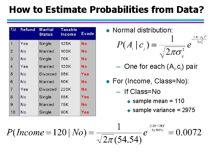
How to Estimate Probabilities from Data? l Normal distribution: – One for each (Ai, ci) pair l For (Income, Class=No): – If Class=No u sample mean = 110 u sample variance = 2975
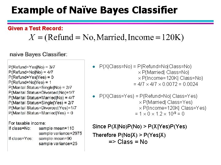
Example of Naïve Bayes Classifier Given a Test Record: l P(X|Class=No) = P(Refund=No|Class=No) P(Married| Class=No) P(Income=120 K| Class=No) = 4/7 0. 0072 = 0. 0024 l P(X|Class=Yes) = P(Refund=No| Class=Yes) P(Married| Class=Yes) P(Income=120 K| Class=Yes) = 1 0 1. 2 10 -9 = 0 Since P(X|No)P(No) > P(X|Yes)P(Yes) Therefore P(No|X) > P(Yes|X) => Class = No
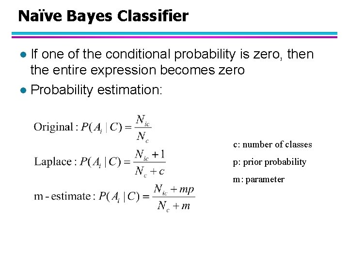
Naïve Bayes Classifier If one of the conditional probability is zero, then the entire expression becomes zero l Probability estimation: l c: number of classes p: prior probability m: parameter
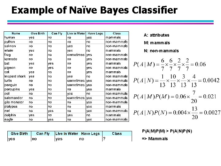
Example of Naïve Bayes Classifier A: attributes M: mammals N: non-mammals P(A|M)P(M) > P(A|N)P(N) => Mammals
Naïve Bayes (Summary) l Robust to isolated noise points l Handle missing values by ignoring the instance during probability estimate calculations l Robust to irrelevant attributes l Independence assumption may not hold for some attributes – Use other techniques such as Bayesian Belief Networks (BBN)
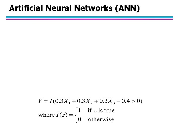
Artificial Neural Networks (ANN) Output Y is 1 if at least two of the three inputs are equal to 1.
Artificial Neural Networks (ANN)
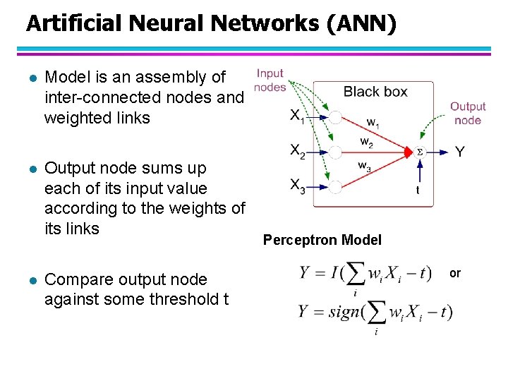
Artificial Neural Networks (ANN) l Model is an assembly of inter-connected nodes and weighted links l Output node sums up each of its input value according to the weights of its links l Compare output node against some threshold t Perceptron Model or
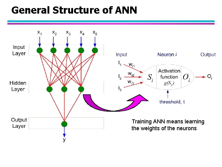
General Structure of ANN Training ANN means learning the weights of the neurons
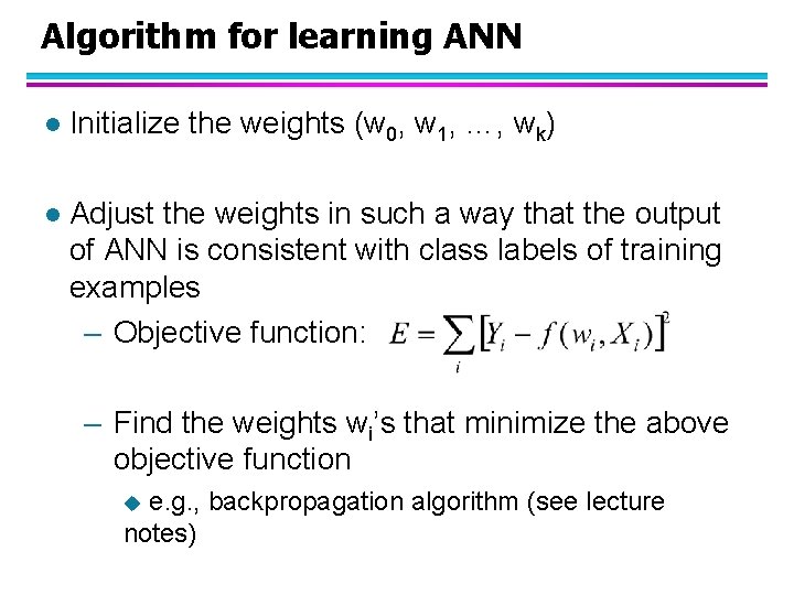
Algorithm for learning ANN l Initialize the weights (w 0, w 1, …, wk) l Adjust the weights in such a way that the output of ANN is consistent with class labels of training examples – Objective function: – Find the weights wi’s that minimize the above objective function e. g. , backpropagation algorithm (see lecture notes) u
Support Vector Machines l Find a linear hyperplane (decision boundary) that will separate the data
Support Vector Machines l One Possible Solution
Support Vector Machines l Another possible solution
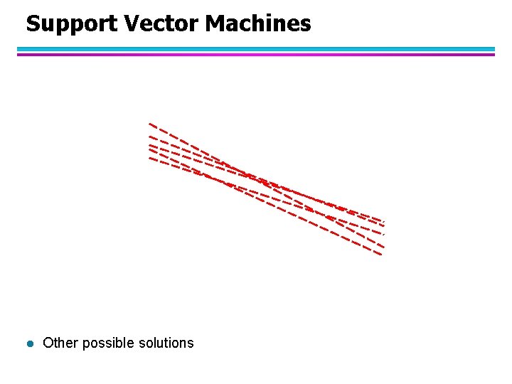
Support Vector Machines l Other possible solutions
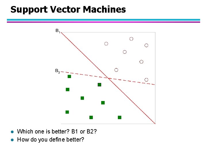
Support Vector Machines l l Which one is better? B 1 or B 2? How do you define better?
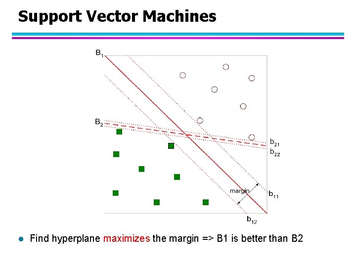
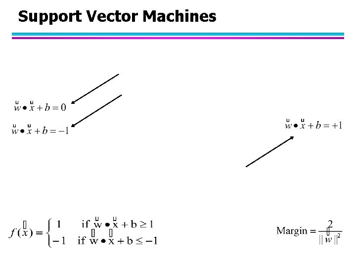
Support Vector Machines l Find hyperplane maximizes the margin => B 1 is better than B 2
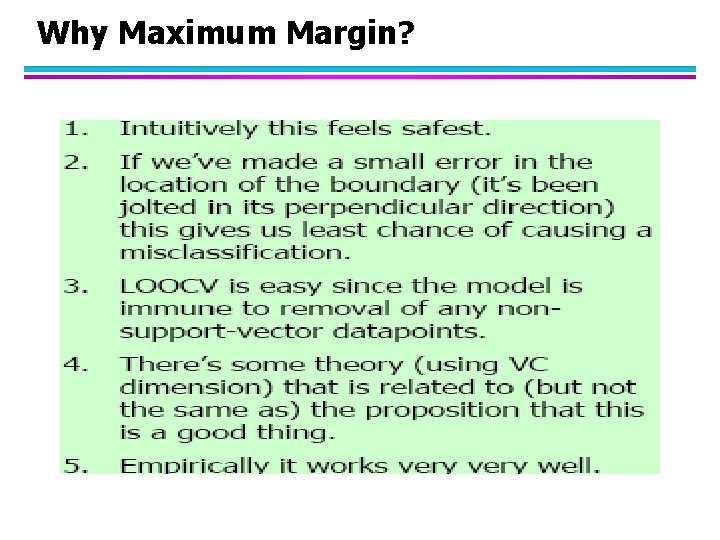
Why Maximum Margin?
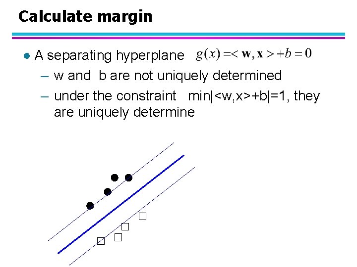
Calculate margin l A separating hyperplane – w and b are not uniquely determined – under the constraint min|<w, x>+b|=1, they are uniquely determine

Calculate margin l the distance between a point x and by |<w, x>+b|/||w|| l thus, the margin is given by 1/||w|| is given
Support Vector Machines
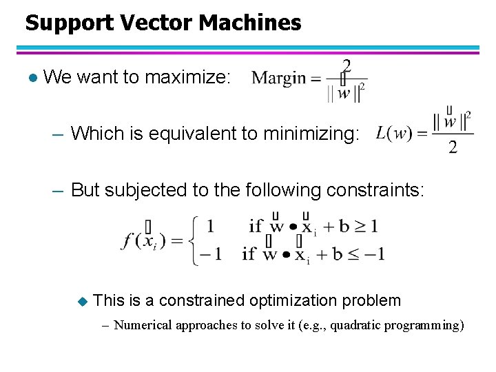
Support Vector Machines l We want to maximize: – Which is equivalent to minimizing: – But subjected to the following constraints: u This is a constrained optimization problem – Numerical approaches to solve it (e. g. , quadratic programming)
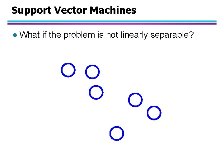
Support Vector Machines l What if the problem is not linearly separable?
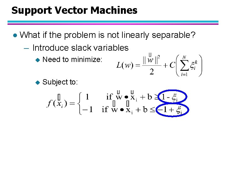
Support Vector Machines l What if the problem is not linearly separable? – Introduce slack variables u Need to minimize: u Subject to:
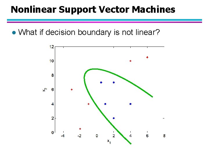
Nonlinear Support Vector Machines l What if decision boundary is not linear?
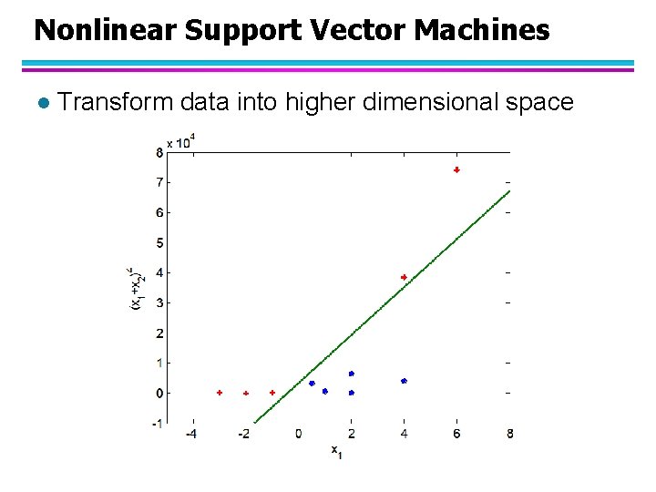
Nonlinear Support Vector Machines l Transform data into higher dimensional space
Ensemble Methods l Construct a set of classifiers from the training data l Predict class label of previously unseen records by aggregating predictions made by multiple classifiers

General Idea
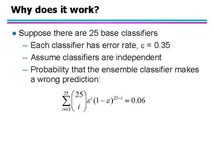
Why does it work? l Suppose there are 25 base classifiers – Each classifier has error rate, = 0. 35 – Assume classifiers are independent – Probability that the ensemble classifier makes a wrong prediction:
Examples of Ensemble Methods l How to generate an ensemble of classifiers? – Bagging – Boosting
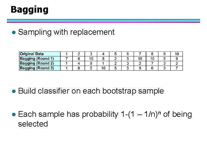
Bagging l Sampling with replacement l Build classifier on each bootstrap sample l Each sample has probability 1 -(1 – 1/n)n of being selected
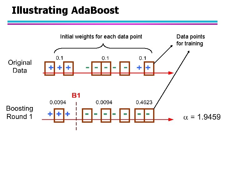
Boosting l An iterative procedure to adaptively change distribution of training data by focusing more on previously misclassified records – Initially, all N records are assigned equal weights – Unlike bagging, weights may change at the end of boosting round
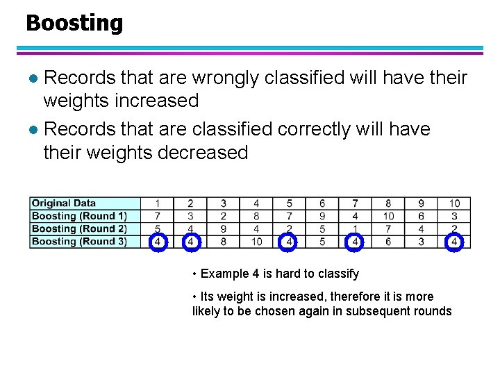
Boosting Records that are wrongly classified will have their weights increased l Records that are classified correctly will have their weights decreased l • Example 4 is hard to classify • Its weight is increased, therefore it is more likely to be chosen again in subsequent rounds
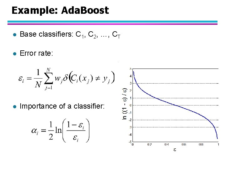
Example: Ada. Boost l Base classifiers: C 1, C 2, …, CT l Error rate: l Importance of a classifier:
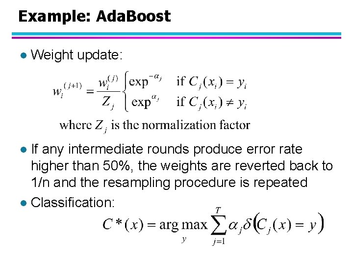
Example: Ada. Boost l Weight update: If any intermediate rounds produce error rate higher than 50%, the weights are reverted back to 1/n and the resampling procedure is repeated l Classification: l
Illustrating Ada. Boost Initial weights for each data point Data points for training
Illustrating Ada. Boost
- Slides: 44