Basis Basics Selected from presentations by Jim Ramsay

Basis Basics Selected from presentations by Jim Ramsay, Mc. Gill University, Hongliang Fei, and Brian Quanz

1. Introduction n Ø Ø Basis: In Linear Algebra, a basis is a set of vectors satisfying: Linear combination of the basis can represent every vector in a given vector space; No element of the set can be represented as a linear combination of the others.

n n n In Function Space, Basis is degenerated to a set of basis functions; Each function in the function space can be represented as a linear combination of the basis functions. Example: Quadratic Polynomial bases {1, t, t^2}

What are basis functions? n n n We need flexible method for constructing a function f(t) that can track local curvature. We pick a system of K basis functions φk(t), and call this the basis for f(t). We express f(t) as a weighted sum of these basis functions: f(t) = a 1φ1(t) + a 2φ2(t) + … + a. KφK(t) The coefficients a 1, … , a. K determine the shape of the function.

What do we want from basis functions? n n n Fast computation of individual basis functions. Flexible: can exhibit the required curvature where needed, but also be nearly linear when appropriate. Fast computation of coefficients ak: possible if matrices of values are diagonal, banded or sparse. Differentiable as required: We make lots of use of derivatives in functional data analysis. Constrained as required, such as periodicity, positivity, monotonicity, asymptotes and etc.

What are some commonly used basis functions? n n n Powers: 1, t, t 2, and so on. They are the basis functions for polynomials. These are not very flexible, and are used only for simple problems. Fourier series: 1, sin(ωt), cos(ωt), sin(2ωt), cos(2ωt), and so on for a fixed known frequency ω. These are used for periodic functions. Spline functions: These have now more or less replaced polynomials for non-periodic problems. More explanation follows.

What is Basis Expansion? n Given data X and transformation Then we model as a linear basis expansion in X, where is a basis function.
 will typically nonlinear in")
Why Basis Expansion? n n n In regression problems, f(X) will typically nonlinear in X; Linear model is convenient and easy to interpret; When sample size is very small but attribute size is very large, linear model is all what we can do to avoid over fitting.

2. Piecewise Polynomials and Splines n Ø Ø n Spline: In Mathematics, a spline is a special function defined piecewise by polynomials; In Computer Science, the term spline more frequently refers to a piecewise polynomial (parametric) curve. Simple construction, ease and accuracy of evaluation, capacity to approximate complex shapes through curve fitting and interactive curve design.
, also X")
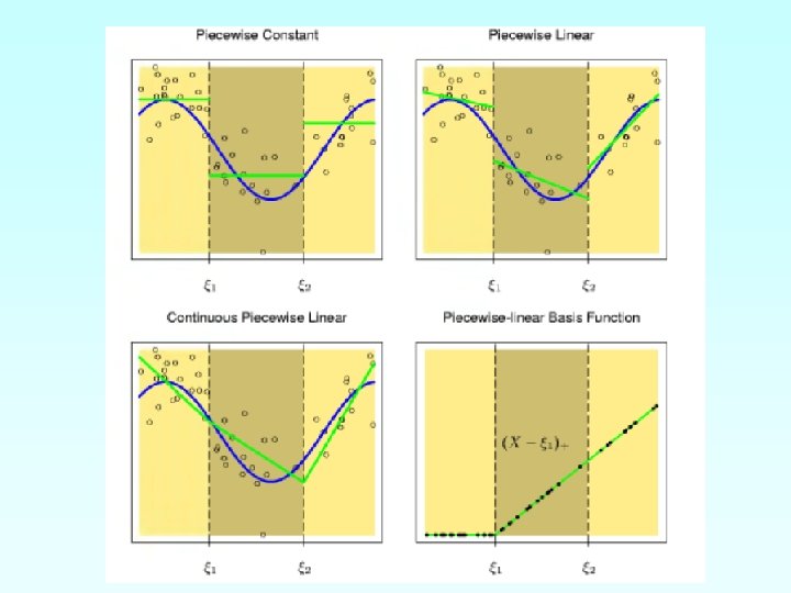
n Assume four knots spline (two boundary knots and two interior knots), also X is one dimensional. Piecewise constant basis: n Piecewise Linear Basis: n

Piecewise Cubic Polynomial n n Basis functions: Six functions corresponding to a sixdimensional linear space.

Piecewise Cubic Polynomial

Spline Interpolation Method Slides taken from the lecture by Authors: Autar Kaw, Jai Paul http: //numericalmethods. eng. usf. edu 14
, (x 1, y 1), ……")
What is Interpolation ? Given (x 0, y 0), (x 1, y 1), …… (xn, yn), find the value of ‘y’ at a value of ‘x’ that is not given. 15 lmethods. eng. usf. edu http: //numerica

Interpolants Polynomials are the most common choice of interpolants because they are easy to: Evaluate Differentiate, and Integrate. 16 lmethods. eng. usf. edu http: //numerica

Why Splines ? 17 lmethods. eng. usf. edu http: //numerica

Why Splines ? 18 Figure : Higher order polynomial interpolation is a bad ideahttp: //numerica lmethods. eng. usf. edu

Linear Interpolation 19 lmethods. eng. usf. edu http: //numerica
 20 lmethods. eng. usf. edu http: //numerica")
Linear Interpolation (contd) 20 lmethods. eng. usf. edu http: //numerica

Example The upward velocity of a rocket is given as a function of time in Table 1. Find the velocity at t=16 seconds using linear splines. Table Velocity as a function of time (s) 0 10 15 20 22. 5 30 21 (m/s) 0 227. 04 362. 78 517. 35 602. 97 901. 67 Figure. Velocity vs. time data for the rocket example lmethods. eng. usf. edu http: //numerica

Linear Interpolation 22 lmethods. eng. usf. edu http: //numerica

Quadratic Interpolation 23 lmethods. eng. usf. edu http: //numerica
 24 lmethods. eng. usf. edu http: //numerica")
Quadratic Interpolation (contd) 24 lmethods. eng. usf. edu http: //numerica
 25 lmethods. eng. usf. edu http: //numerica")
Quadratic Splines (contd) 25 lmethods. eng. usf. edu http: //numerica
 26 lmethods. eng. usf. edu http: //numerica")
Quadratic Splines (contd) 26 lmethods. eng. usf. edu http: //numerica
 27 lmethods. eng. usf. edu http: //numerica")
Quadratic Splines (contd) 27 lmethods. eng. usf. edu http: //numerica

Quadratic Spline Example The upward velocity of a rocket is given as a function of time. Using quadratic splines a) Find the velocity at t=16 seconds b) Find the acceleration at t=16 seconds c) Find the distance covered between t=11 and t=16 seconds Table Velocity as a function of time (s) 0 10 15 20 22. 5 30 28 (m/s) 0 227. 04 362. 78 517. 35 602. 97 901. 67 Figure. Velocity vs. time data for the rocket example lmethods. eng. usf. edu http: //numerica

Solution Let us set up the equations 29 lmethods. eng. usf. edu http: //numerica

Each Spline Goes Through Two Consecutive Data Points 30 lmethods. eng. usf. edu http: //numerica
")
Each Spline Goes Through Two Consecutive Data Points 31 t s 0 10 v(t) m/s 0 227. 04 15 20 22. 5 30 362. 78 517. 35 602. 97 901. 67 lmethods. eng. usf. edu http: //numerica

Derivatives are Continuous at Interior Data Points 32 lmethods. eng. usf. edu http: //numerica

Derivatives are continuous at Interior Data Points At t=10 At t=15 At t=20 At t=22. 5 33 lmethods. eng. usf. edu http: //numerica

Last Equation 34 lmethods. eng. usf. edu http: //numerica

Final Set of Equations 35 lmethods. eng. usf. edu http: //numerica

Coefficients of Spline 36 i ai bi ci 1 0 22. 704 0 2 0. 8888 4. 928 88. 88 3 − 0. 1356 35. 66 − 141. 61 4 1. 6048 5 0. 20889 − 33. 956 554. 55 28. 86 − 152. 13 lmethods. eng. usf. edu http: //numerica

Quadratic Spline Interpolation Part 2 of 2 http: //numericalmethods. eng. usf. edu 37 lmethods. eng. usf. edu http: //numerica

Final Solution 38 lmethods. eng. usf. edu http: //numerica
 Velocity at t=16 39 lmethods. eng. usf. edu")
Velocity at a Particular Point a) Velocity at t=16 39 lmethods. eng. usf. edu http: //numerica

Quadratic Spline Graph t=a: 2: b;

Quadratic Spline Graph t=a: 0. 5: b;

Natural Cubic Spline Interpolation SPLINE OF DEGREE k = 3 n n n The domain of S is an interval [a, b]. S, S’’ are all continuous functions on [a, b]. There are points ti (the knots of S) such that a = t 0 < t 1 <. . tn = b and such that S is a polynomial of degree at most k on each subinterval [t i, ti+1]. x t 0 t 1 … tn y y 0 y 1 … yn ti are knots
 is a cubic polynomial that will be used on")
Natural Cubic Spline Interpolation Si(x) is a cubic polynomial that will be used on the subinterval [ xi, xi+1 ].
 = aix 3 + bix 2 + cix")
Natural Cubic Spline Interpolation n Si(x) = aix 3 + bix 2 + cix + di • • 4 Coefficients with n subintervals = 4 n equations There are 4 n-2 conditions • Interpolation conditions Continuity conditions • Natural Conditions • • • S’’(x 0) = 0 S’’(xn) = 0
- Slides: 44