Basics of Statistical Data Analysis Quantum Universe Lecture

Basics of Statistical Data Analysis Quantum Universe Lecture DESY / U. Hamburg Zoom / 13 April 2021 https: //indico. desy. de/event/29561/ Glen Cowan Physics Department Royal Holloway, University of London g. cowan@rhul. ac. uk www. pp. rhul. ac. uk/~cowan G. Cowan / RHUL Physics DESY / U. Hamburg Basics of Statistical Data Analysis 1

Outline • Basic introduction to frequentist vs Bayesian approaches • Basics of fitting, hypothesis tests and asymptotics • Treating systematic uncertainties with nuisance parameters Everything here is a subset of the University of London course: http: //www. pp. rhul. ac. uk/~cowan/stat_course. html G. Cowan / RHUL Physics DESY / U. Hamburg Basics of Statistical Data Analysis 2

Some statistics books, papers, etc. G. Cowan, Statistical Data Analysis, Clarendon, Oxford, 1998 R. J. Barlow, Statistics: A Guide to the Use of Statistical Methods in the Physical Sciences, Wiley, 1989 Ilya Narsky and Frank C. Porter, Statistical Analysis Techniques in Particle Physics, Wiley, 2014. Luca Lista, Statistical Methods for Data Analysis in Particle Physics, Springer, 2017. L. Lyons, Statistics for Nuclear and Particle Physics, CUP, 1986 F. James. , Statistical and Computational Methods in Experimental Physics, 2 nd ed. , World Scientific, 2006 S. Brandt, Statistical and Computational Methods in Data Analysis, Springer, New York, 1998. P. A. Zyla et al. (Particle Data Group), Prog. Theor. Exp. Phys. 2020, 083 C 01 (2020); pdg. lbl. gov sections on probability, statistics, MC. G. Cowan / RHUL Physics DESY / U. Hamburg Basics of Statistical Data Analysis 3

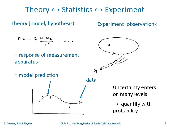
Theory ↔ Statistics ↔ Experiment Theory (model, hypothesis): Experiment (observation): + response of measurement apparatus = model prediction data Uncertainty enters on many levels → quantify with probability G. Cowan / RHUL Physics DESY / U. Hamburg Basics of Statistical Data Analysis 4

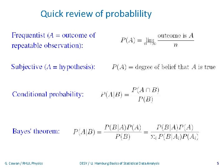
Quick review of probablility G. Cowan / RHUL Physics DESY / U. Hamburg Basics of Statistical Data Analysis 5

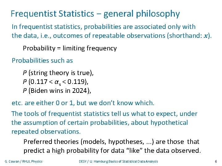
Frequentist Statistics − general philosophy In frequentist statistics, probabilities are associated only with the data, i. e. , outcomes of repeatable observations (shorthand: x). Probability = limiting frequency Probabilities such as P (string theory is true), P (0. 117 < αs < 0. 119), P (Biden wins in 2024), etc. are either 0 or 1, but we don’t know which. The tools of frequentist statistics tell us what to expect, under the assumption of certain probabilities, about hypothetical repeated observations. Preferred theories (models, hypotheses, . . . ) are those that predict a high probability for data “like” the data observed. G. Cowan / RHUL Physics DESY / U. Hamburg Basics of Statistical Data Analysis 6

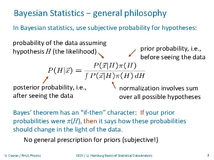
Bayesian Statistics − general philosophy In Bayesian statistics, use subjective probability for hypotheses: probability of the data assuming hypothesis H (the likelihood) posterior probability, i. e. , after seeing the data prior probability, i. e. , before seeing the data normalization involves sum over all possible hypotheses Bayes’ theorem has an “if-then” character: If your prior probabilities were π(H), then it says how these probabilities should change in the light of the data. No general prescription for priors (subjective!) G. Cowan / RHUL Physics DESY / U. Hamburg Basics of Statistical Data Analysis 7

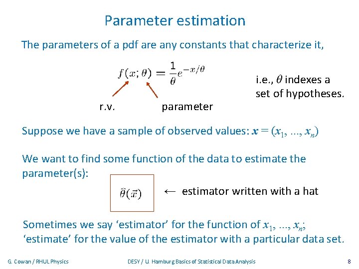
Parameter estimation The parameters of a pdf are any constants that characterize it, r. v. parameter i. e. , θ indexes a set of hypotheses. Suppose we have a sample of observed values: x = (x 1, . . . , xn) We want to find some function of the data to estimate the parameter(s): ← estimator written with a hat Sometimes we say ‘estimator’ for the function of x 1, . . . , xn; ‘estimate’ for the value of the estimator with a particular data set. G. Cowan / RHUL Physics DESY / U. Hamburg Basics of Statistical Data Analysis 8

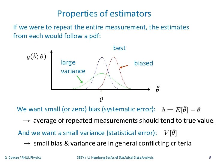
Properties of estimators If we were to repeat the entire measurement, the estimates from each would follow a pdf: best large variance biased We want small (or zero) bias (systematic error): → average of repeated measurements should tend to true value. And we want a small variance (statistical error): → small bias & variance are in general conflicting criteria G. Cowan / RHUL Physics DESY / U. Hamburg Basics of Statistical Data Analysis 9

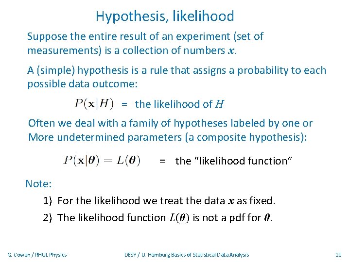
Hypothesis, likelihood Suppose the entire result of an experiment (set of measurements) is a collection of numbers x. A (simple) hypothesis is a rule that assigns a probability to each possible data outcome: = the likelihood of H Often we deal with a family of hypotheses labeled by one or More undetermined parameters (a composite hypothesis): = the “likelihood function” Note: 1) For the likelihood we treat the data x as fixed. 2) The likelihood function L(θ) is not a pdf for θ. G. Cowan / RHUL Physics DESY / U. Hamburg Basics of Statistical Data Analysis 10

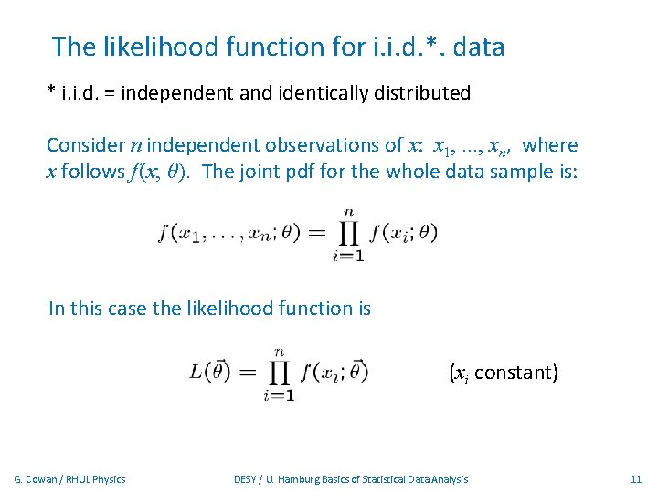
The likelihood function for i. i. d. *. data * i. i. d. = independent and identically distributed Consider n independent observations of x: x 1, . . . , xn, where x follows f (x; θ). The joint pdf for the whole data sample is: In this case the likelihood function is (xi constant) G. Cowan / RHUL Physics DESY / U. Hamburg Basics of Statistical Data Analysis 11

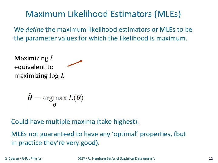
Maximum Likelihood Estimators (MLEs) We define the maximum likelihood estimators or MLEs to be the parameter values for which the likelihood is maximum. Maximizing L equivalent to maximizing log L Could have multiple maxima (take highest). MLEs not guaranteed to have any ‘optimal’ properties, (but in practice they’re very good). G. Cowan / RHUL Physics DESY / U. Hamburg Basics of Statistical Data Analysis 12

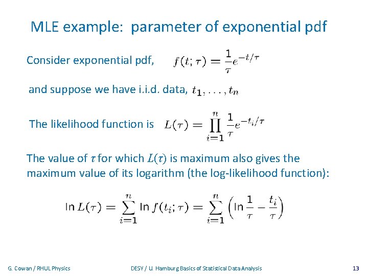
MLE example: parameter of exponential pdf Consider exponential pdf, and suppose we have i. i. d. data, The likelihood function is The value of τ for which L(τ) is maximum also gives the maximum value of its logarithm (the log-likelihood function): G. Cowan / RHUL Physics DESY / U. Hamburg Basics of Statistical Data Analysis 13

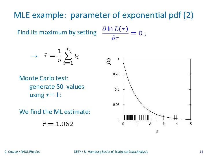
MLE example: parameter of exponential pdf (2) Find its maximum by setting → Monte Carlo test: generate 50 values using τ = 1: We find the ML estimate: G. Cowan / RHUL Physics DESY / U. Hamburg Basics of Statistical Data Analysis 14

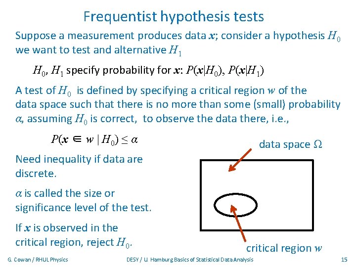
Frequentist hypothesis tests Suppose a measurement produces data x; consider a hypothesis H 0 we want to test and alternative H 1 H 0, H 1 specify probability for x: P(x|H 0), P(x|H 1) A test of H 0 is defined by specifying a critical region w of the data space such that there is no more than some (small) probability α, assuming H 0 is correct, to observe the data there, i. e. , P(x ∈ w | H 0) ≤ α data space Ω Need inequality if data are discrete. α is called the size or significance level of the test. If x is observed in the critical region, reject H 0. G. Cowan / RHUL Physics critical region w DESY / U. Hamburg Basics of Statistical Data Analysis 15

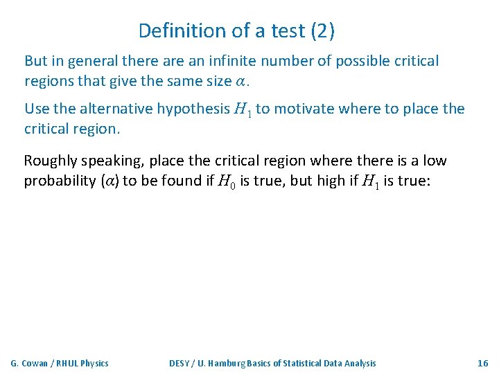
Definition of a test (2) But in general there an infinite number of possible critical regions that give the same size α. Use the alternative hypothesis H 1 to motivate where to place the critical region. Roughly speaking, place the critical region where there is a low probability (α) to be found if H 0 is true, but high if H 1 is true: G. Cowan / RHUL Physics DESY / U. Hamburg Basics of Statistical Data Analysis 16

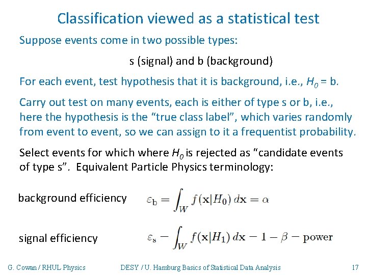
Classification viewed as a statistical test Suppose events come in two possible types: s (signal) and b (background) For each event, test hypothesis that it is background, i. e. , H 0 = b. Carry out test on many events, each is either of type s or b, i. e. , here the hypothesis is the “true class label”, which varies randomly from event to event, so we can assign to it a frequentist probability. Select events for which where H 0 is rejected as “candidate events of type s”. Equivalent Particle Physics terminology: background efficiency signal efficiency G. Cowan / RHUL Physics DESY / U. Hamburg Basics of Statistical Data Analysis 17

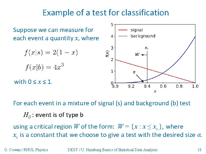
Example of a test for classification Suppose we can measure for each event a quantity x, where with 0 ≤ x ≤ 1. For each event in a mixture of signal (s) and background (b) test H 0 : event is of type b using a critical region W of the form: W = { x : x ≤ xc }, where xc is a constant that we choose to give a test with the desired size α. G. Cowan / RHUL Physics DESY / U. Hamburg Basics of Statistical Data Analysis 18

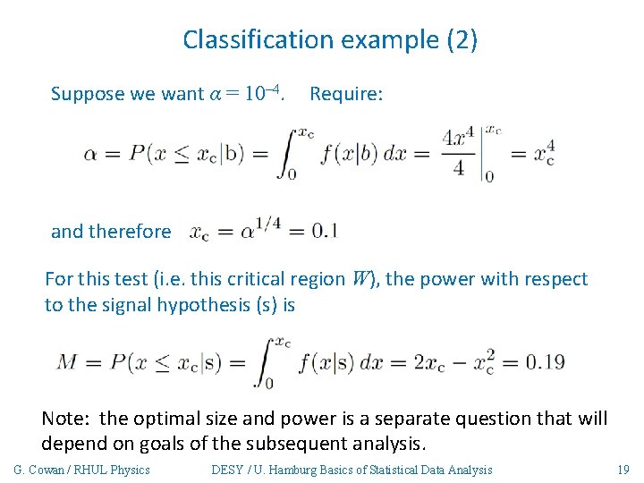
Classification example (2) Suppose we want α = 10 -4. Require: and therefore For this test (i. e. this critical region W), the power with respect to the signal hypothesis (s) is Note: the optimal size and power is a separate question that will depend on goals of the subsequent analysis. G. Cowan / RHUL Physics DESY / U. Hamburg Basics of Statistical Data Analysis 19

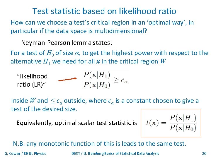
Test statistic based on likelihood ratio How can we choose a test’s critical region in an ‘optimal way’, in particular if the data space is multidimensional? Neyman-Pearson lemma states: For a test of H 0 of size α, to get the highest power with respect to the alternative H 1 we need for all x in the critical region W ”likelihood ratio (LR)” inside W and ≤ cα outside, where cα is a constant chosen to give a test of the desired size. Equivalently, optimal scalar test statistic is N. B. any monotonic function of this is leads to the same test. G. Cowan / RHUL Physics DESY / U. Hamburg Basics of Statistical Data Analysis 20

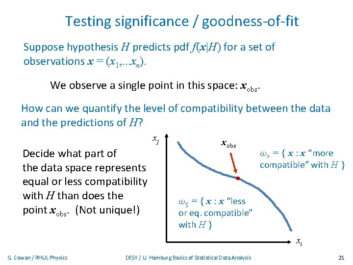
Testing significance / goodness-of-fit Suppose hypothesis H predicts pdf f (x|H) for a set of observations x = (x 1, . . . xn). We observe a single point in this space: xobs. How can we quantify the level of compatibility between the data and the predictions of H? xj Decide what part of the data space represents equal or less compatibility with H than does the point xobs. (Not unique!) xobs ω> = { x : x “more compatible” with H } ω≤ = { x : x “less or eq. compatible” with H } xi G. Cowan / RHUL Physics DESY / U. Hamburg Basics of Statistical Data Analysis 21

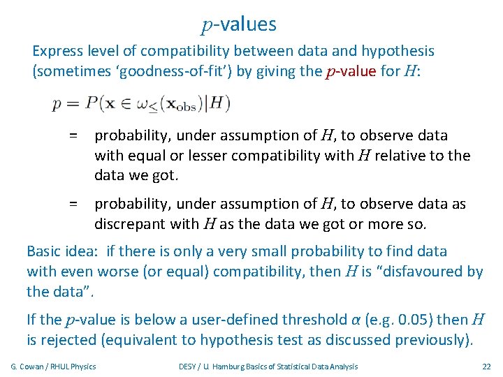
p-values Express level of compatibility between data and hypothesis (sometimes ‘goodness-of-fit’) by giving the p-value for H: = probability, under assumption of H, to observe data with equal or lesser compatibility with H relative to the data we got. = probability, under assumption of H, to observe data as discrepant with H as the data we got or more so. Basic idea: if there is only a very small probability to find data with even worse (or equal) compatibility, then H is “disfavoured by the data”. If the p-value is below a user-defined threshold α (e. g. 0. 05) then H is rejected (equivalent to hypothesis test as discussed previously). G. Cowan / RHUL Physics DESY / U. Hamburg Basics of Statistical Data Analysis 22

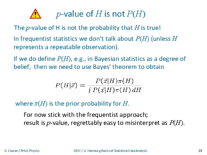
p-value of H is not P(H) The p-value of H is not the probability that H is true! In frequentist statistics we don’t talk about P(H) (unless H represents a repeatable observation). If we do define P(H), e. g. , in Bayesian statistics as a degree of belief, then we need to use Bayes’ theorem to obtain where π(H) is the prior probability for H. For now stick with the frequentist approach; result is p-value, regrettably easy to misinterpret as P(H). G. Cowan / RHUL Physics DESY / U. Hamburg Basics of Statistical Data Analysis 23

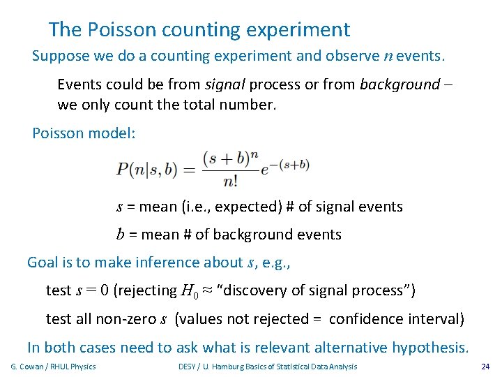
The Poisson counting experiment Suppose we do a counting experiment and observe n events. Events could be from signal process or from background – we only count the total number. Poisson model: s = mean (i. e. , expected) # of signal events b = mean # of background events Goal is to make inference about s, e. g. , test s = 0 (rejecting H 0 ≈ “discovery of signal process”) test all non-zero s (values not rejected = confidence interval) In both cases need to ask what is relevant alternative hypothesis. G. Cowan / RHUL Physics DESY / U. Hamburg Basics of Statistical Data Analysis 24

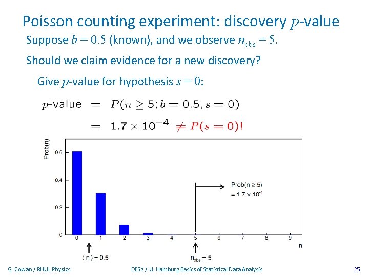
Poisson counting experiment: discovery p-value Suppose b = 0. 5 (known), and we observe nobs = 5. Should we claim evidence for a new discovery? Give p-value for hypothesis s = 0: G. Cowan / RHUL Physics DESY / U. Hamburg Basics of Statistical Data Analysis 25

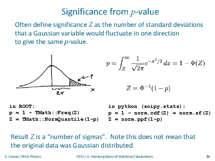
Significance from p-value Often define significance Z as the number of standard deviations that a Gaussian variable would fluctuate in one direction to give the same p-value. in ROOT: p = 1 - TMath: : Freq(Z) Z = TMath: : Norm. Quantile(1 -p) in python (scipy. stats): p = 1 - norm. cdf(Z) = norm. sf(Z) Z = norm. ppf(1 -p) Result Z is a “number of sigmas”. Note this does not mean that the original data was Gaussian distributed. G. Cowan / RHUL Physics DESY / U. Hamburg Basics of Statistical Data Analysis 26

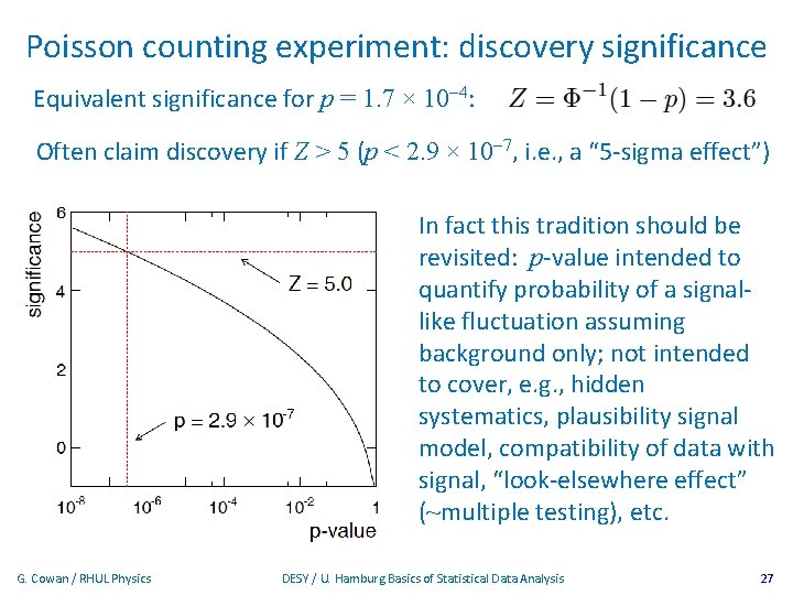
Poisson counting experiment: discovery significance Equivalent significance for p = 1. 7 × 10 -4: Often claim discovery if Z > 5 (p < 2. 9 × 10 -7, i. e. , a “ 5 -sigma effect”) In fact this tradition should be revisited: p-value intended to quantify probability of a signallike fluctuation assuming background only; not intended to cover, e. g. , hidden systematics, plausibility signal model, compatibility of data with signal, “look-elsewhere effect” (~multiple testing), etc. G. Cowan / RHUL Physics DESY / U. Hamburg Basics of Statistical Data Analysis 27

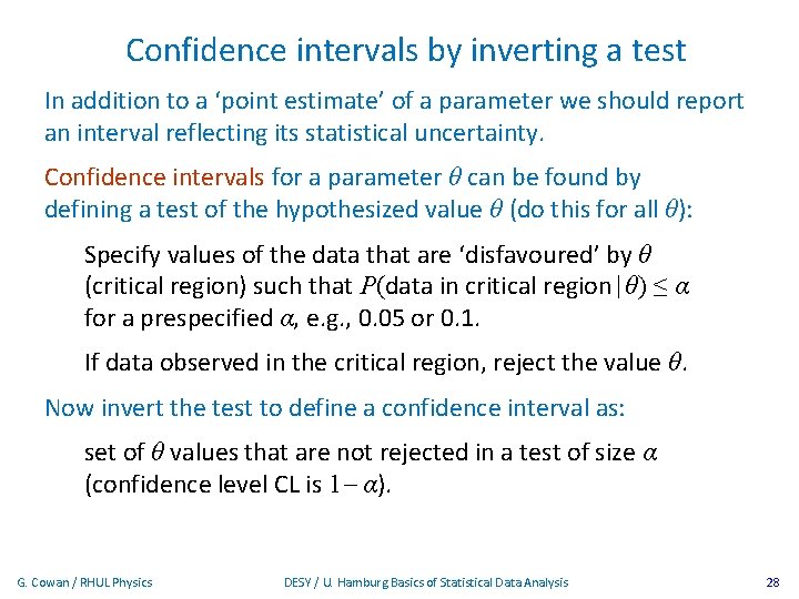
Confidence intervals by inverting a test In addition to a ‘point estimate’ of a parameter we should report an interval reflecting its statistical uncertainty. Confidence intervals for a parameter θ can be found by defining a test of the hypothesized value θ (do this for all θ): Specify values of the data that are ‘disfavoured’ by θ (critical region) such that P(data in critical region|θ) ≤ α for a prespecified α, e. g. , 0. 05 or 0. 1. If data observed in the critical region, reject the value θ. Now invert the test to define a confidence interval as: set of θ values that are not rejected in a test of size α (confidence level CL is 1 - α). G. Cowan / RHUL Physics DESY / U. Hamburg Basics of Statistical Data Analysis 28

Relation between confidence interval and p-value Equivalently we can consider a significance test for each hypothesized value of θ, resulting in a p-value, pθ. If pθ ≤ α, then we reject θ. The confidence interval at CL = 1 – α consists of those values of θ that are not rejected. E. g. an upper limit on θ is the greatest value for which pθ > α. In practice find by setting pθ = α and solve for θ. For a multidimensional parameter space θ = (θ 1, . . . θM) use same idea – result is a confidence “region” with boundary determined by pθ = α. G. Cowan / RHUL Physics DESY / U. Hamburg Basics of Statistical Data Analysis 29

Coverage probability of confidence interval If the true value of θ is rejected, then it’s not in the confidence interval. The probability for this is by construction (equality for continuous data): P(reject θ|θ) ≤ α = type-I error rate Therefore, the probability for the interval to contain or “cover” θ is P(conf. interval “covers” θ|θ) ≥ 1 – α This assumes that the set of θ values considered includes the true value, i. e. , it assumes the composite hypothesis P(x|H, θ). G. Cowan / RHUL Physics DESY / U. Hamburg Basics of Statistical Data Analysis 30

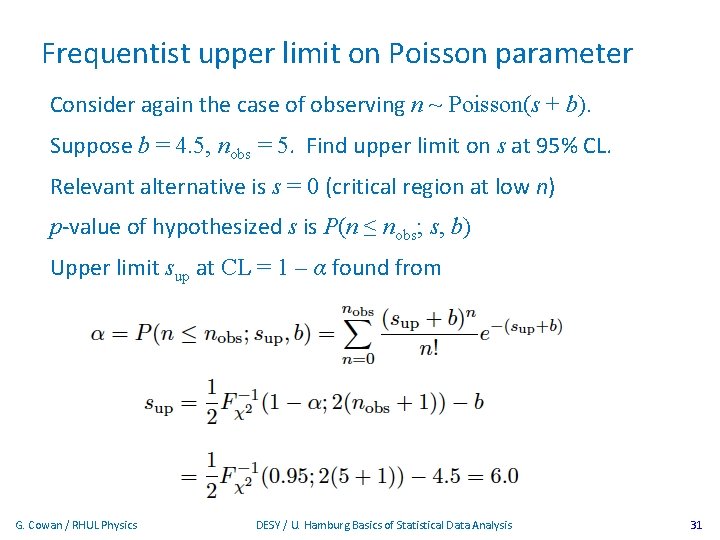
Frequentist upper limit on Poisson parameter Consider again the case of observing n ~ Poisson(s + b). Suppose b = 4. 5, nobs = 5. Find upper limit on s at 95% CL. Relevant alternative is s = 0 (critical region at low n) p-value of hypothesized s is P(n ≤ nobs; s, b) Upper limit sup at CL = 1 – α found from G. Cowan / RHUL Physics DESY / U. Hamburg Basics of Statistical Data Analysis 31

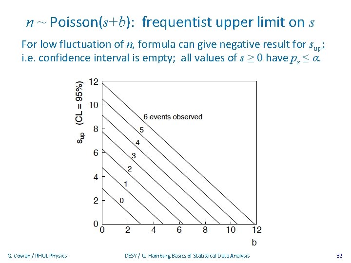
n ~ Poisson(s+b): frequentist upper limit on s For low fluctuation of n, formula can give negative result for sup; i. e. confidence interval is empty; all values of s ≥ 0 have ps ≤ α. G. Cowan / RHUL Physics DESY / U. Hamburg Basics of Statistical Data Analysis 32

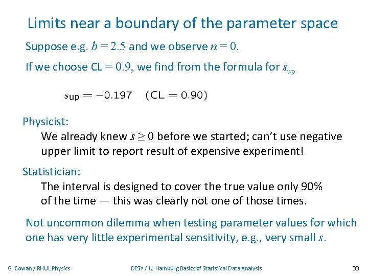
Limits near a boundary of the parameter space Suppose e. g. b = 2. 5 and we observe n = 0. If we choose CL = 0. 9, we find from the formula for sup Physicist: We already knew s ≥ 0 before we started; can’t use negative upper limit to report result of expensive experiment! Statistician: The interval is designed to cover the true value only 90% of the time — this was clearly not one of those times. Not uncommon dilemma when testing parameter values for which one has very little experimental sensitivity, e. g. , very small s. G. Cowan / RHUL Physics DESY / U. Hamburg Basics of Statistical Data Analysis 33

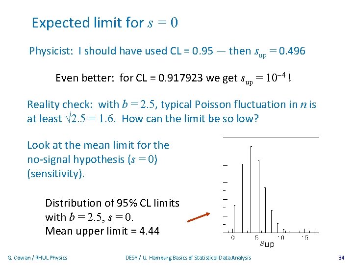
Expected limit for s = 0 Physicist: I should have used CL = 0. 95 — then sup = 0. 496 Even better: for CL = 0. 917923 we get sup = 10 -4 ! Reality check: with b = 2. 5, typical Poisson fluctuation in n is at least √ 2. 5 = 1. 6. How can the limit be so low? Look at the mean limit for the no-signal hypothesis (s = 0) (sensitivity). Distribution of 95% CL limits with b = 2. 5, s = 0. Mean upper limit = 4. 44 G. Cowan / RHUL Physics DESY / U. Hamburg Basics of Statistical Data Analysis 34

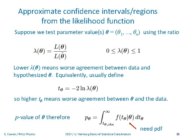
Approximate confidence intervals/regions from the likelihood function Suppose we test parameter value(s) θ = (θ 1, . . . , θn) using the ratio Lower λ(θ) means worse agreement between data and hypothesized θ. Equivalently, usually define so higher tθ means worse agreement between θ and the data. p-value of θ therefore G. Cowan / RHUL Physics DESY / U. Hamburg Basics of Statistical Data Analysis need pdf 35

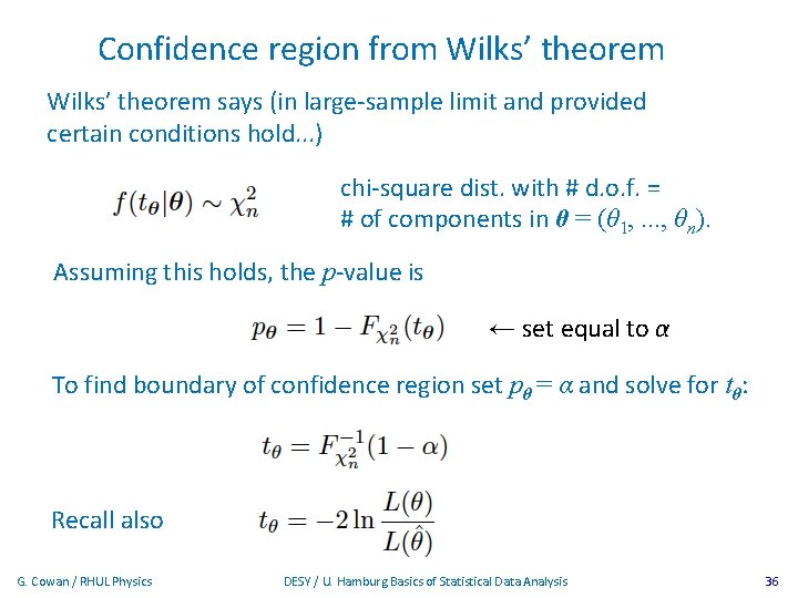
Confidence region from Wilks’ theorem says (in large-sample limit and provided certain conditions hold. . . ) chi-square dist. with # d. o. f. = # of components in θ = (θ 1, . . . , θn). Assuming this holds, the p-value is ← set equal to α To find boundary of confidence region set pθ = α and solve for tθ: Recall also G. Cowan / RHUL Physics DESY / U. Hamburg Basics of Statistical Data Analysis 36

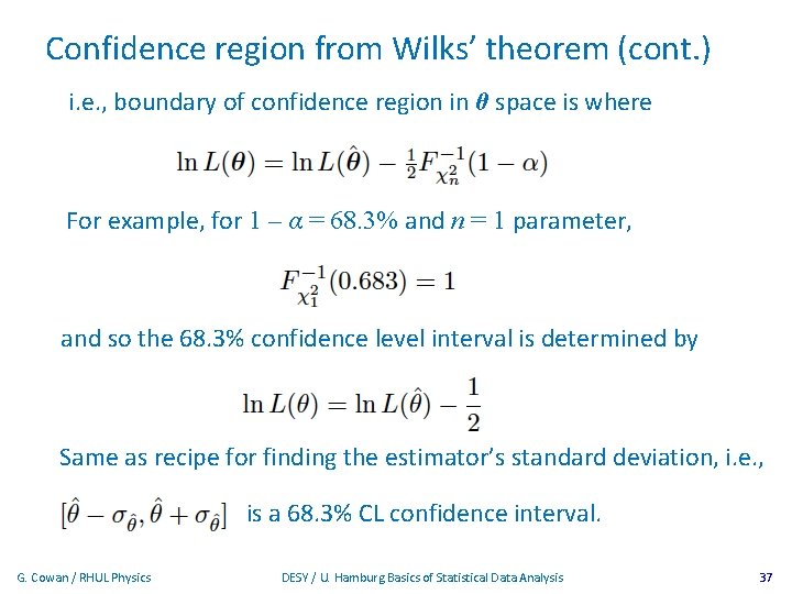
Confidence region from Wilks’ theorem (cont. ) i. e. , boundary of confidence region in θ space is where For example, for 1 – α = 68. 3% and n = 1 parameter, and so the 68. 3% confidence level interval is determined by Same as recipe for finding the estimator’s standard deviation, i. e. , is a 68. 3% CL confidence interval. G. Cowan / RHUL Physics DESY / U. Hamburg Basics of Statistical Data Analysis 37

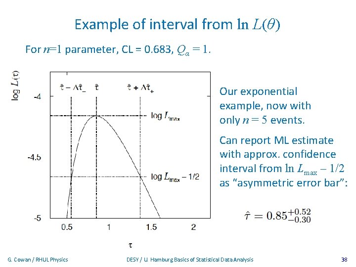
Example of interval from ln L(θ) For n=1 parameter, CL = 0. 683, Qα = 1. Our exponential example, now with only n = 5 events. Can report ML estimate with approx. confidence interval from ln Lmax – 1/2 as “asymmetric error bar”: G. Cowan / RHUL Physics DESY / U. Hamburg Basics of Statistical Data Analysis 38

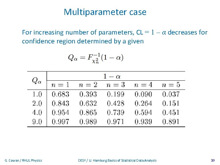
Multiparameter case For increasing number of parameters, CL = 1 – α decreases for confidence region determined by a given G. Cowan / RHUL Physics DESY / U. Hamburg Basics of Statistical Data Analysis 39

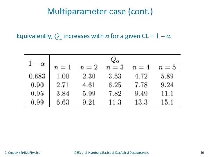
Multiparameter case (cont. ) Equivalently, Qα increases with n for a given CL = 1 – α. G. Cowan / RHUL Physics DESY / U. Hamburg Basics of Statistical Data Analysis 40

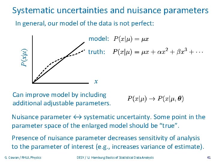
Systematic uncertainties and nuisance parameters In general, our model of the data is not perfect: P (x|μ) model: truth: x Can improve model by including additional adjustable parameters. Nuisance parameter ↔ systematic uncertainty. Some point in the parameter space of the enlarged model should be “true”. Presence of nuisance parameter decreases sensitivity of analysis to the parameter of interest (e. g. , increases variance of estimate). G. Cowan / RHUL Physics DESY / U. Hamburg Basics of Statistical Data Analysis 41

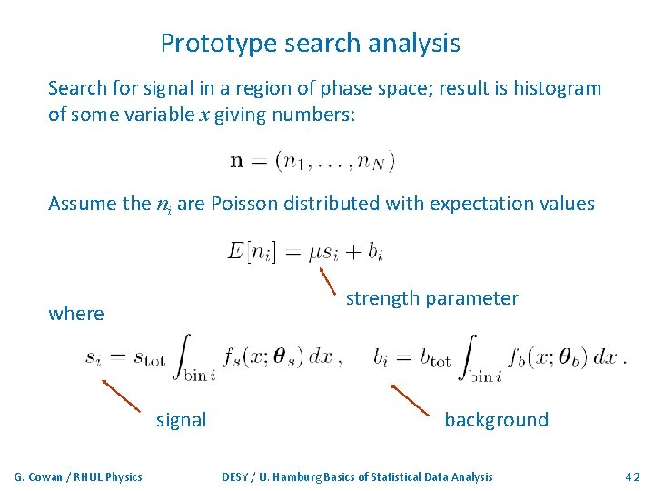
Prototype search analysis Search for signal in a region of phase space; result is histogram of some variable x giving numbers: Assume the ni are Poisson distributed with expectation values strength parameter where signal G. Cowan / RHUL Physics background DESY / U. Hamburg Basics of Statistical Data Analysis 42

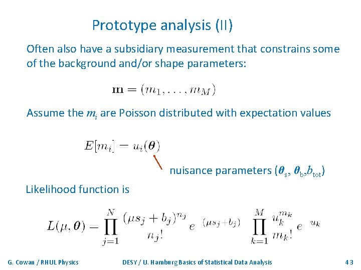
Prototype analysis (II) Often also have a subsidiary measurement that constrains some of the background and/or shape parameters: Assume the mi are Poisson distributed with expectation values nuisance parameters (θs, θb, btot) Likelihood function is G. Cowan / RHUL Physics DESY / U. Hamburg Basics of Statistical Data Analysis 43

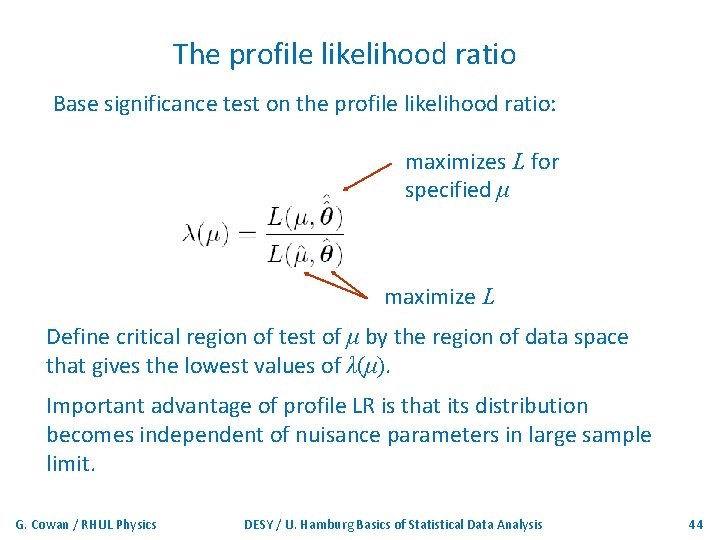
The profile likelihood ratio Base significance test on the profile likelihood ratio: maximizes L for specified μ maximize L Define critical region of test of μ by the region of data space that gives the lowest values of λ(μ). Important advantage of profile LR is that its distribution becomes independent of nuisance parameters in large sample limit. G. Cowan / RHUL Physics DESY / U. Hamburg Basics of Statistical Data Analysis 44

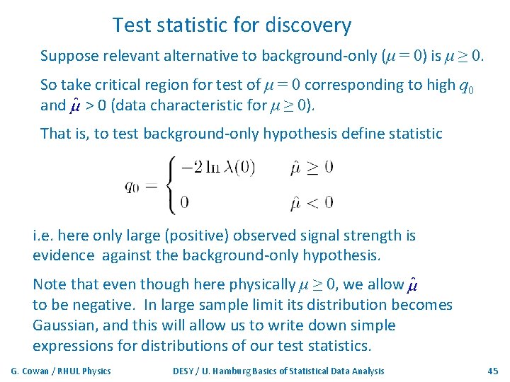
Test statistic for discovery Suppose relevant alternative to background-only (μ = 0) is μ ≥ 0. So take critical region for test of μ = 0 corresponding to high q 0 and > 0 (data characteristic for μ ≥ 0). That is, to test background-only hypothesis define statistic i. e. here only large (positive) observed signal strength is evidence against the background-only hypothesis. Note that even though here physically μ ≥ 0, we allow to be negative. In large sample limit its distribution becomes Gaussian, and this will allow us to write down simple expressions for distributions of our test statistics. G. Cowan / RHUL Physics DESY / U. Hamburg Basics of Statistical Data Analysis 45

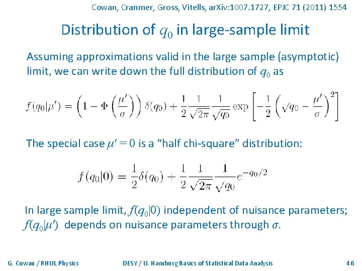
Cowan, Cranmer, Gross, Vitells, ar. Xiv: 1007. 1727, EPJC 71 (2011) 1554 Distribution of q 0 in large-sample limit Assuming approximations valid in the large sample (asymptotic) limit, we can write down the full distribution of q 0 as The special case μ′ = 0 is a “half chi-square” distribution: In large sample limit, f (q 0|0) independent of nuisance parameters; f (q 0|μ′) depends on nuisance parameters through σ. G. Cowan / RHUL Physics DESY / U. Hamburg Basics of Statistical Data Analysis 46

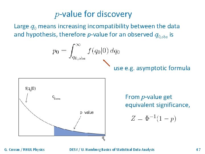
p-value for discovery Large q 0 means increasing incompatibility between the data and hypothesis, therefore p-value for an observed q 0, obs is use e. g. asymptotic formula From p-value get equivalent significance, G. Cowan / RHUL Physics DESY / U. Hamburg Basics of Statistical Data Analysis 47

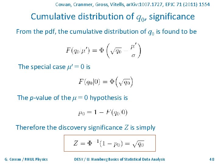
Cowan, Cranmer, Gross, Vitells, ar. Xiv: 1007. 1727, EPJC 71 (2011) 1554 Cumulative distribution of q 0, significance From the pdf, the cumulative distribution of q 0 is found to be The special case μ′ = 0 is The p-value of the μ = 0 hypothesis is Therefore the discovery significance Z is simply G. Cowan / RHUL Physics DESY / U. Hamburg Basics of Statistical Data Analysis 48

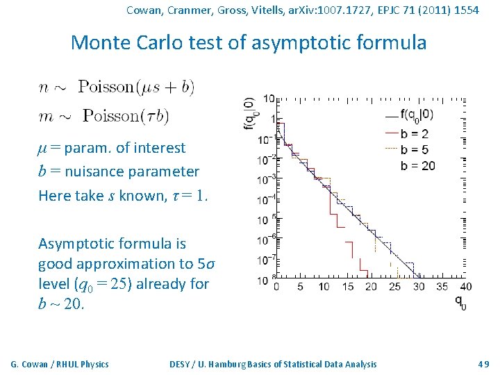
Cowan, Cranmer, Gross, Vitells, ar. Xiv: 1007. 1727, EPJC 71 (2011) 1554 Monte Carlo test of asymptotic formula μ = param. of interest b = nuisance parameter Here take s known, τ = 1. Asymptotic formula is good approximation to 5σ level (q 0 = 25) already for b ~ 20. G. Cowan / RHUL Physics DESY / U. Hamburg Basics of Statistical Data Analysis 49

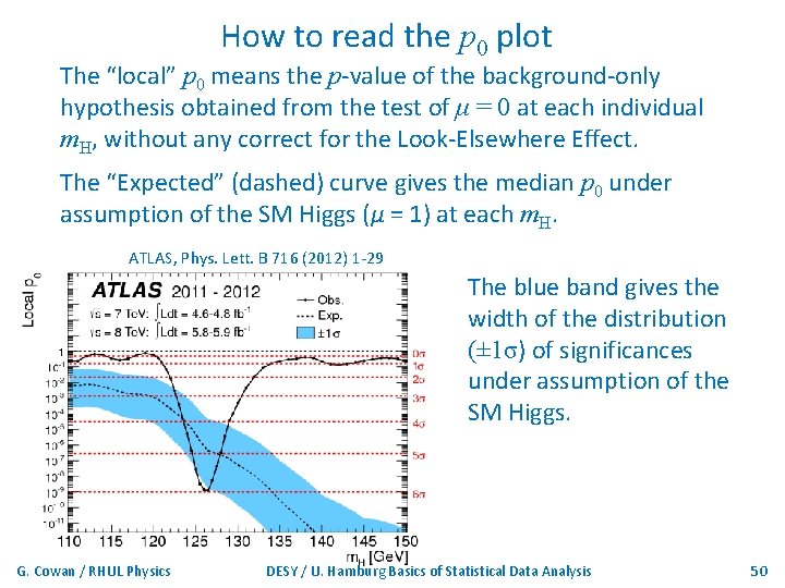
How to read the p 0 plot The “local” p 0 means the p-value of the background-only hypothesis obtained from the test of μ = 0 at each individual m. H, without any correct for the Look-Elsewhere Effect. The “Expected” (dashed) curve gives the median p 0 under assumption of the SM Higgs (μ = 1) at each m. H. ATLAS, Phys. Lett. B 716 (2012) 1 -29 The blue band gives the width of the distribution (± 1σ) of significances under assumption of the SM Higgs. G. Cowan / RHUL Physics DESY / U. Hamburg Basics of Statistical Data Analysis 50

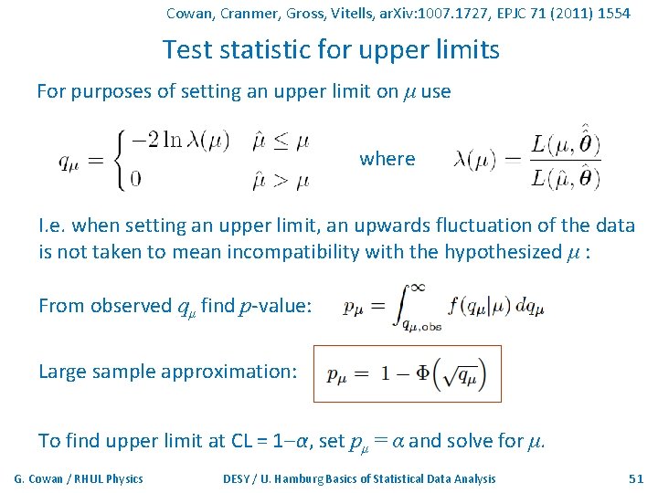
Cowan, Cranmer, Gross, Vitells, ar. Xiv: 1007. 1727, EPJC 71 (2011) 1554 Test statistic for upper limits For purposes of setting an upper limit on μ use where I. e. when setting an upper limit, an upwards fluctuation of the data is not taken to mean incompatibility with the hypothesized μ : From observed qμ find p-value: Large sample approximation: To find upper limit at CL = 1 -α, set pμ = α and solve for μ. G. Cowan / RHUL Physics DESY / U. Hamburg Basics of Statistical Data Analysis 51

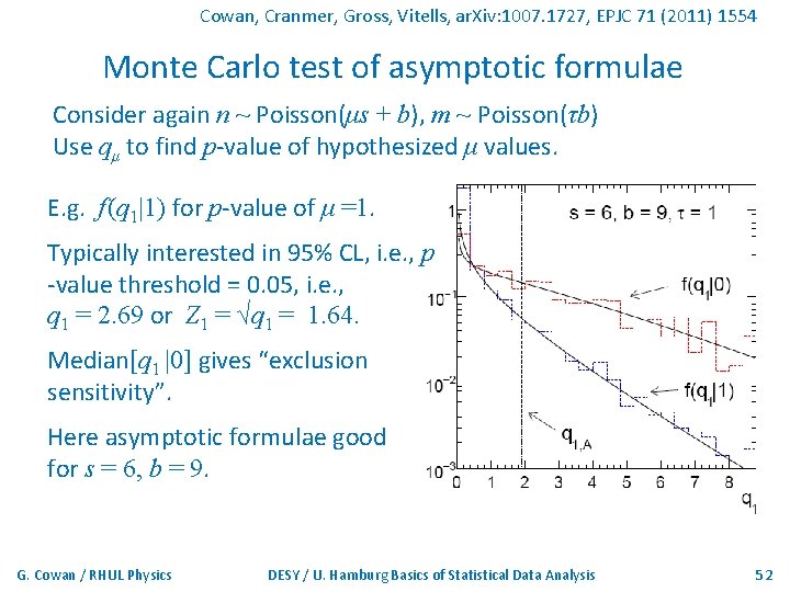
Cowan, Cranmer, Gross, Vitells, ar. Xiv: 1007. 1727, EPJC 71 (2011) 1554 Monte Carlo test of asymptotic formulae Consider again n ~ Poisson(μs + b), m ~ Poisson(τb) Use qμ to find p-value of hypothesized μ values. E. g. f (q 1|1) for p-value of μ =1. Typically interested in 95% CL, i. e. , p -value threshold = 0. 05, i. e. , q 1 = 2. 69 or Z 1 = √q 1 = 1. 64. Median[q 1 |0] gives “exclusion sensitivity”. Here asymptotic formulae good for s = 6, b = 9. G. Cowan / RHUL Physics DESY / U. Hamburg Basics of Statistical Data Analysis 52

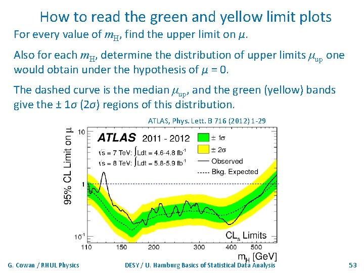
How to read the green and yellow limit plots For every value of m. H, find the upper limit on μ. Also for each m. H, determine the distribution of upper limits μup one would obtain under the hypothesis of μ = 0. The dashed curve is the median μup, and the green (yellow) bands give the ± 1σ (2σ) regions of this distribution. ATLAS, Phys. Lett. B 716 (2012) 1 -29 G. Cowan / RHUL Physics DESY / U. Hamburg Basics of Statistical Data Analysis 53

Finally One lecture only enough for a brief introduction to: Parameter estimation, maximum likelihood Hypothesis tests, p-values Limits (confidence intervals/regions) Systematics (nuisance parameters) Asymptotics (Wilks’ theorem) Final thought: once the basic formalism is fixed, most of the work focuses on writing down the likelihood, e. g. , P(x|θ), and including in it enough parameters to adequately describe the data (true for both Bayesian and frequentist approaches). G. Cowan / RHUL Physics DESY / U. Hamburg Basics of Statistical Data Analysis 54

Extra slides G. Cowan / RHUL Physics DESY / U. Hamburg Basics of Statistical Data Analysis 55

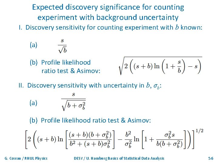
Expected discovery significance for counting experiment with background uncertainty I. Discovery sensitivity for counting experiment with b known: (a) (b) Profile likelihood ratio test & Asimov: II. Discovery sensitivity with uncertainty in b, σb: (a) (b) Profile likelihood ratio test & Asimov: G. Cowan / RHUL Physics DESY / U. Hamburg Basics of Statistical Data Analysis 56

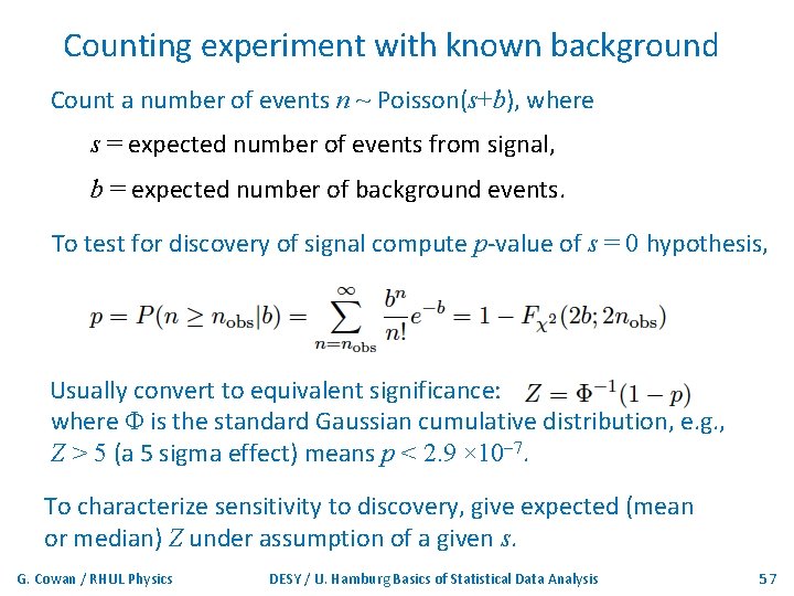
Counting experiment with known background Count a number of events n ~ Poisson(s+b), where s = expected number of events from signal, b = expected number of background events. To test for discovery of signal compute p-value of s = 0 hypothesis, Usually convert to equivalent significance: where Φ is the standard Gaussian cumulative distribution, e. g. , Z > 5 (a 5 sigma effect) means p < 2. 9 × 10 -7. To characterize sensitivity to discovery, give expected (mean or median) Z under assumption of a given s. G. Cowan / RHUL Physics DESY / U. Hamburg Basics of Statistical Data Analysis 57

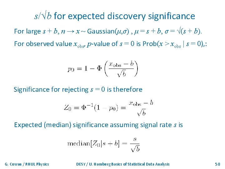
s/√b for expected discovery significance For large s + b, n → x ~ Gaussian(μ, σ) , μ = s + b, σ = √(s + b). For observed value xobs, p-value of s = 0 is Prob(x > xobs | s = 0), : Significance for rejecting s = 0 is therefore Expected (median) significance assuming signal rate s is G. Cowan / RHUL Physics DESY / U. Hamburg Basics of Statistical Data Analysis 58

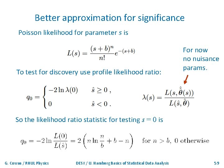
Better approximation for significance Poisson likelihood for parameter s is To test for discovery use profile likelihood ratio: For now no nuisance params. So the likelihood ratio statistic for testing s = 0 is G. Cowan / RHUL Physics DESY / U. Hamburg Basics of Statistical Data Analysis 59

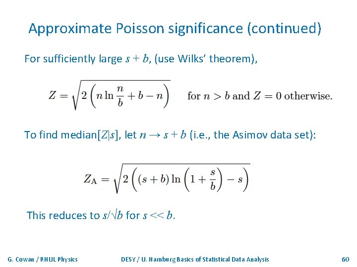
Approximate Poisson significance (continued) For sufficiently large s + b, (use Wilks’ theorem), To find median[Z|s], let n → s + b (i. e. , the Asimov data set): This reduces to s/√b for s << b. G. Cowan / RHUL Physics DESY / U. Hamburg Basics of Statistical Data Analysis 60

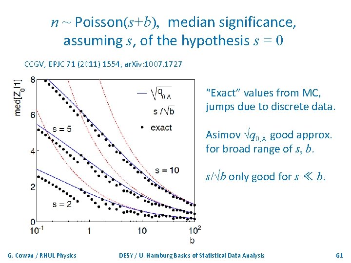
n ~ Poisson(s+b), median significance, assuming s, of the hypothesis s = 0 CCGV, EPJC 71 (2011) 1554, ar. Xiv: 1007. 1727 “Exact” values from MC, jumps due to discrete data. Asimov √q 0, A good approx. for broad range of s, b. s/√b only good for s ≪ b. G. Cowan / RHUL Physics DESY / U. Hamburg Basics of Statistical Data Analysis 61

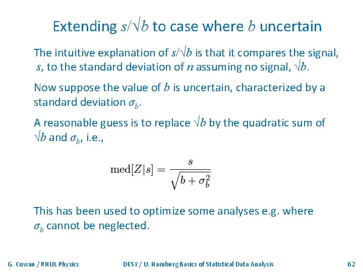
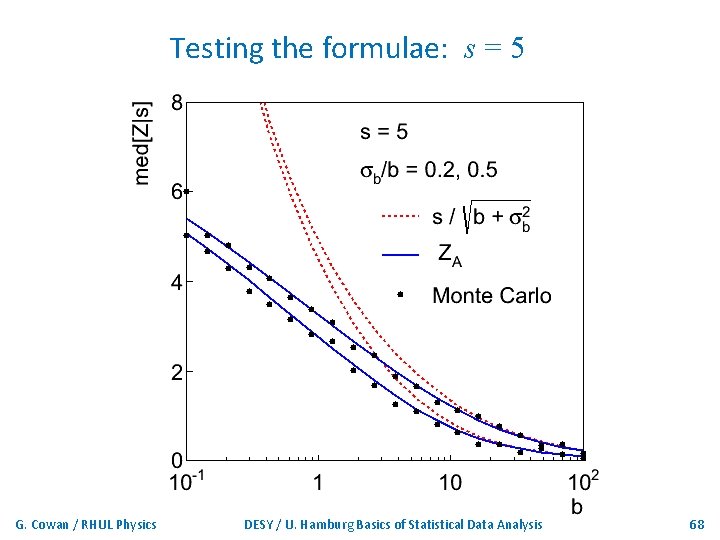
Extending s/√b to case where b uncertain The intuitive explanation of s/√b is that it compares the signal, s, to the standard deviation of n assuming no signal, √b. Now suppose the value of b is uncertain, characterized by a standard deviation σb. A reasonable guess is to replace √b by the quadratic sum of √b and σb, i. e. , This has been used to optimize some analyses e. g. where σb cannot be neglected. G. Cowan / RHUL Physics DESY / U. Hamburg Basics of Statistical Data Analysis 62

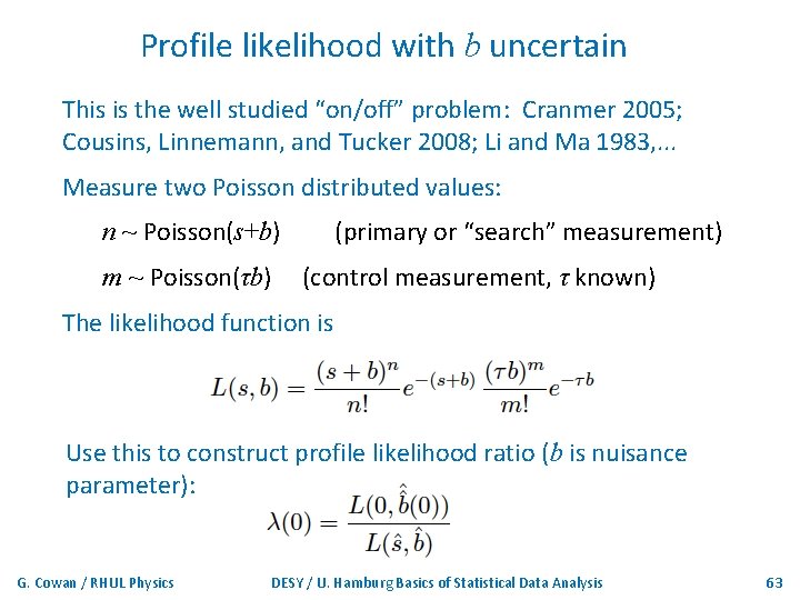
Profile likelihood with b uncertain This is the well studied “on/off” problem: Cranmer 2005; Cousins, Linnemann, and Tucker 2008; Li and Ma 1983, . . . Measure two Poisson distributed values: n ~ Poisson(s+b) m ~ Poisson(τb) (primary or “search” measurement) (control measurement, τ known) The likelihood function is Use this to construct profile likelihood ratio (b is nuisance parameter): G. Cowan / RHUL Physics DESY / U. Hamburg Basics of Statistical Data Analysis 63

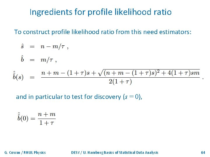
Ingredients for profile likelihood ratio To construct profile likelihood ratio from this need estimators: and in particular to test for discovery (s = 0), G. Cowan / RHUL Physics DESY / U. Hamburg Basics of Statistical Data Analysis 64

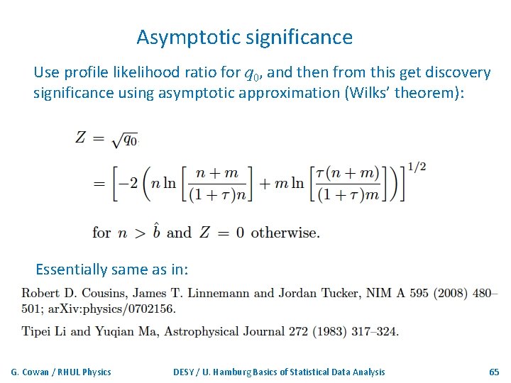
Asymptotic significance Use profile likelihood ratio for q 0, and then from this get discovery significance using asymptotic approximation (Wilks’ theorem): Essentially same as in: G. Cowan / RHUL Physics DESY / U. Hamburg Basics of Statistical Data Analysis 65

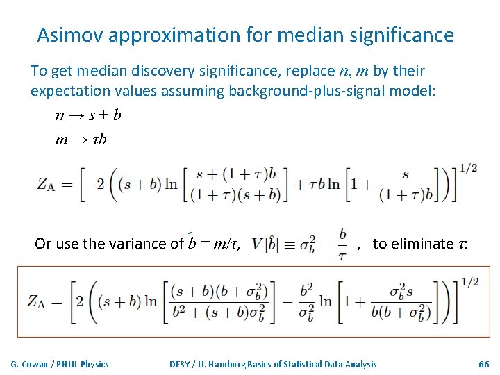
Asimov approximation for median significance To get median discovery significance, replace n, m by their expectation values assuming background-plus-signal model: n→s+b m → τb Or use the variance of ˆb = m/τ, G. Cowan / RHUL Physics , to eliminate τ: DESY / U. Hamburg Basics of Statistical Data Analysis 66

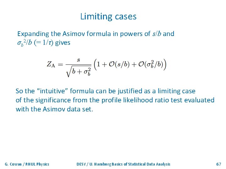
Limiting cases Expanding the Asimov formula in powers of s/b and σb 2/b (= 1/τ) gives So the “intuitive” formula can be justified as a limiting case of the significance from the profile likelihood ratio test evaluated with the Asimov data set. G. Cowan / RHUL Physics DESY / U. Hamburg Basics of Statistical Data Analysis 67

Testing the formulae: s = 5 G. Cowan / RHUL Physics DESY / U. Hamburg Basics of Statistical Data Analysis 68

Using sensitivity to optimize a cut G. Cowan / RHUL Physics DESY / U. Hamburg Basics of Statistical Data Analysis 69

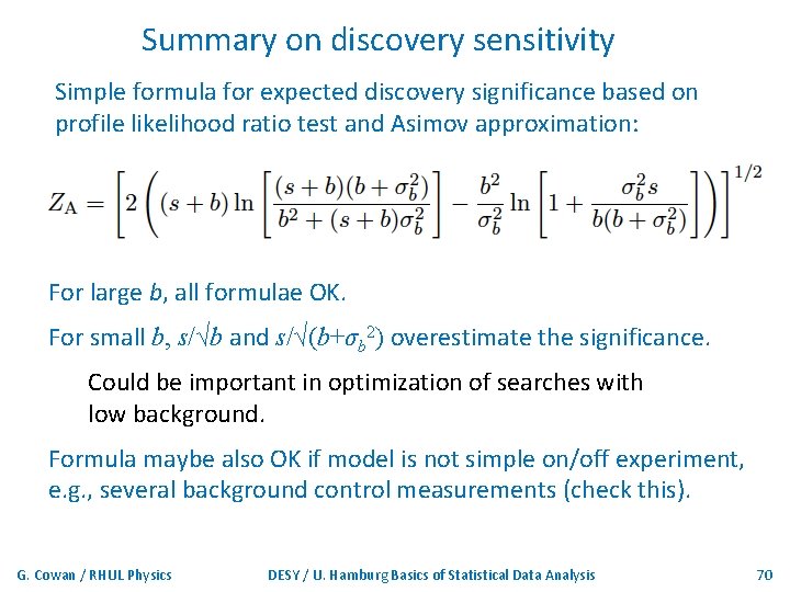
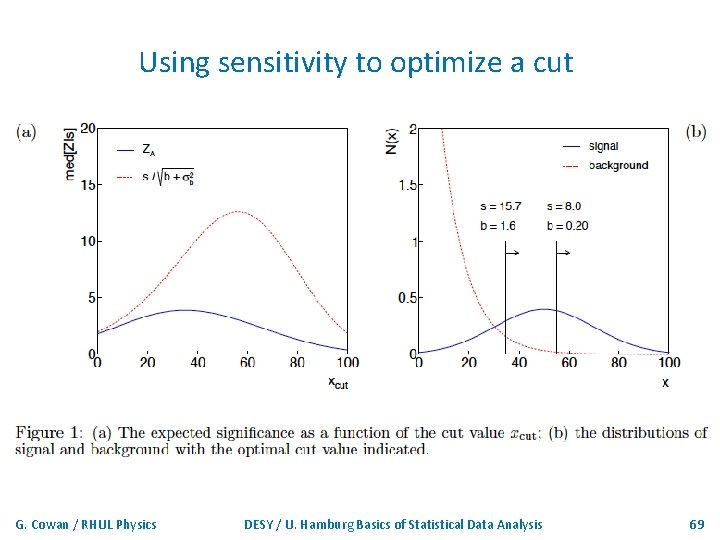
Summary on discovery sensitivity Simple formula for expected discovery significance based on profile likelihood ratio test and Asimov approximation: For large b, all formulae OK. For small b, s/√b and s/√(b+σb 2) overestimate the significance. Could be important in optimization of searches with low background. Formula maybe also OK if model is not simple on/off experiment, e. g. , several background control measurements (check this). G. Cowan / RHUL Physics DESY / U. Hamburg Basics of Statistical Data Analysis 70

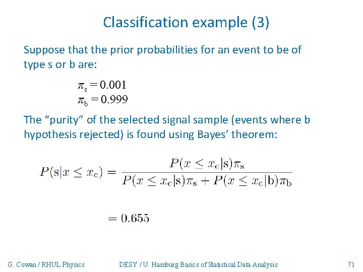
Classification example (3) Suppose that the prior probabilities for an event to be of type s or b are: πs = 0. 001 πb = 0. 999 The “purity” of the selected signal sample (events where b hypothesis rejected) is found using Bayes’ theorem: G. Cowan / RHUL Physics DESY / U. Hamburg Basics of Statistical Data Analysis 71

Large-sample (asymptotic) properties of MLEs Suppose we have an i. i. d. data sample of size n: x 1, . . . , xn In the large-sample (or “asymptotic”) limit (n → ∞) and assuming regularity conditions one can show that the likelihood and MLE have several important properties. The regularity conditions include: • the boundaries of the data space cannot depend on the parameter; • the parameter cannot be on the edge of the parameter space; • ln L(θ) must be differentiable; ^ • the only solution to �� ln L/�� θ = 0 is θ. In the slides immediately following the properties are shown without proof for a single parameter; the corresponding properties hold also for the multiparameter case, θ = (θ 1, . . . , θm). G. Cowan / RHUL Physics DESY / U. Hamburg Basics of Statistical Data Analysis 72

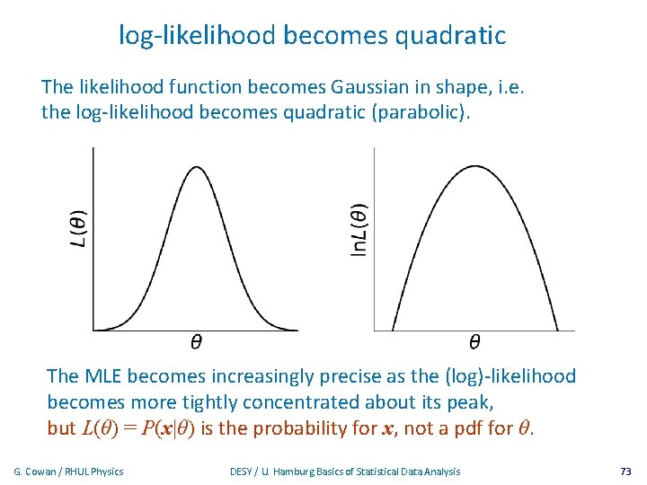
log-likelihood becomes quadratic The likelihood function becomes Gaussian in shape, i. e. the log-likelihood becomes quadratic (parabolic). The MLE becomes increasingly precise as the (log)-likelihood becomes more tightly concentrated about its peak, but L(θ) = P(x|θ) is the probability for x, not a pdf for θ. G. Cowan / RHUL Physics DESY / U. Hamburg Basics of Statistical Data Analysis 73

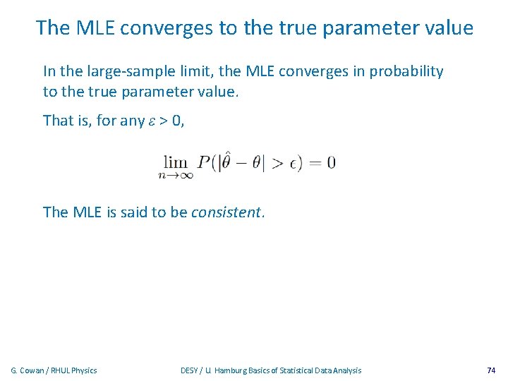
The MLE converges to the true parameter value In the large-sample limit, the MLE converges in probability to the true parameter value. That is, for any ε > 0, The MLE is said to be consistent. G. Cowan / RHUL Physics DESY / U. Hamburg Basics of Statistical Data Analysis 74

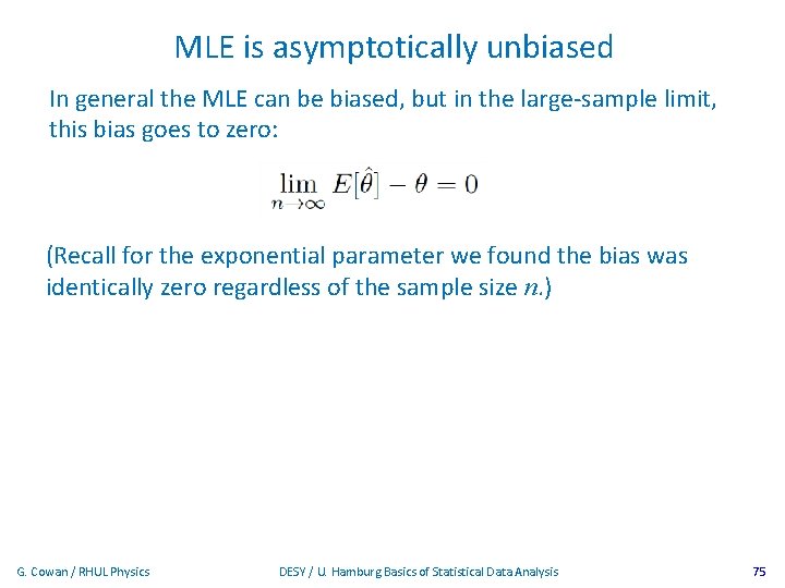
MLE is asymptotically unbiased In general the MLE can be biased, but in the large-sample limit, this bias goes to zero: (Recall for the exponential parameter we found the bias was identically zero regardless of the sample size n. ) G. Cowan / RHUL Physics DESY / U. Hamburg Basics of Statistical Data Analysis 75

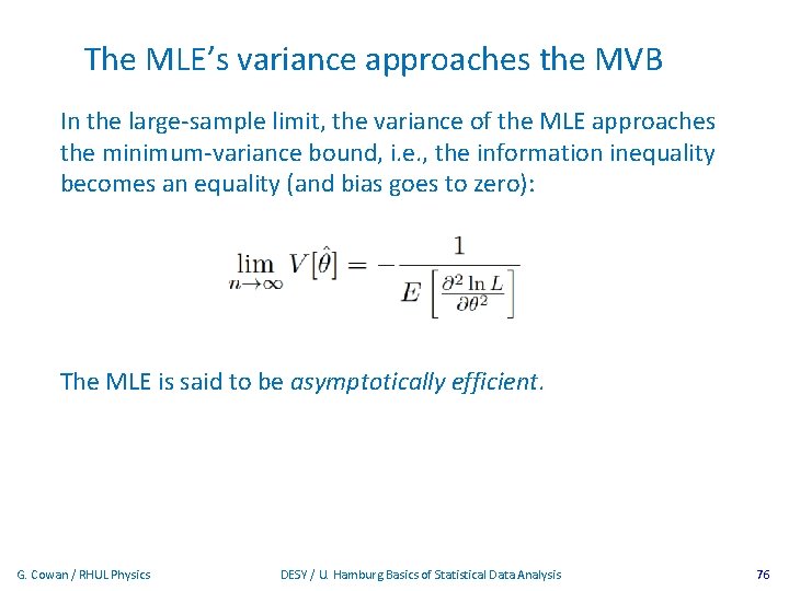
The MLE’s variance approaches the MVB In the large-sample limit, the variance of the MLE approaches the minimum-variance bound, i. e. , the information inequality becomes an equality (and bias goes to zero): The MLE is said to be asymptotically efficient. G. Cowan / RHUL Physics DESY / U. Hamburg Basics of Statistical Data Analysis 76

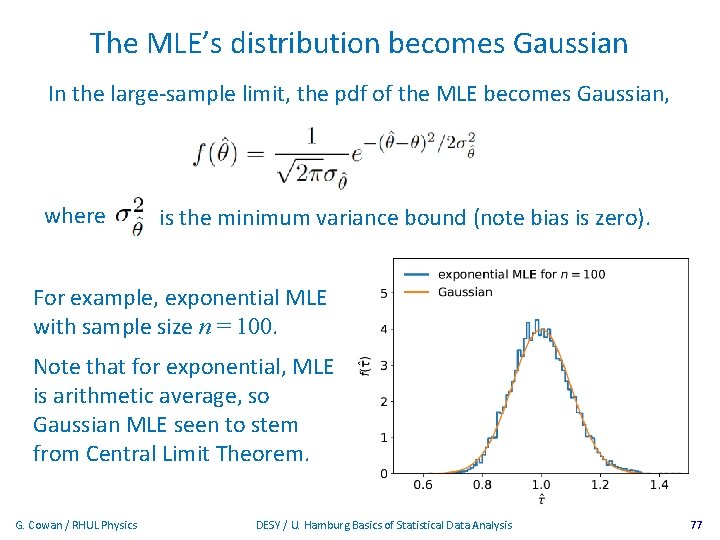
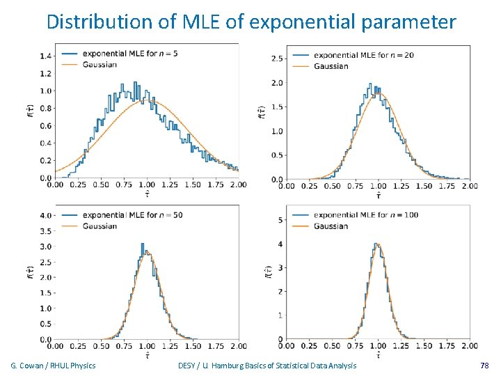
The MLE’s distribution becomes Gaussian In the large-sample limit, the pdf of the MLE becomes Gaussian, where is the minimum variance bound (note bias is zero). For example, exponential MLE with sample size n = 100. Note that for exponential, MLE is arithmetic average, so Gaussian MLE seen to stem from Central Limit Theorem. G. Cowan / RHUL Physics DESY / U. Hamburg Basics of Statistical Data Analysis 77

Distribution of MLE of exponential parameter G. Cowan / RHUL Physics DESY / U. Hamburg Basics of Statistical Data Analysis 78

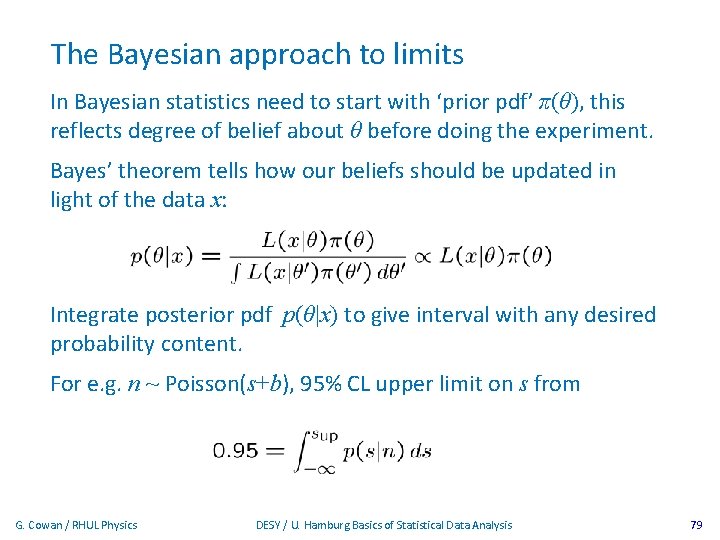
The Bayesian approach to limits In Bayesian statistics need to start with ‘prior pdf’ π(θ), this reflects degree of belief about θ before doing the experiment. Bayes’ theorem tells how our beliefs should be updated in light of the data x: Integrate posterior pdf p(θ|x) to give interval with any desired probability content. For e. g. n ~ Poisson(s+b), 95% CL upper limit on s from G. Cowan / RHUL Physics DESY / U. Hamburg Basics of Statistical Data Analysis 79

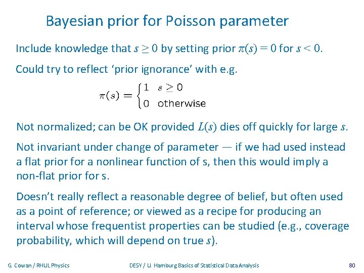
Bayesian prior for Poisson parameter Include knowledge that s ≥ 0 by setting prior π(s) = 0 for s < 0. Could try to reflect ‘prior ignorance’ with e. g. Not normalized; can be OK provided L(s) dies off quickly for large s. Not invariant under change of parameter — if we had used instead a flat prior for a nonlinear function of s, then this would imply a non-flat prior for s. Doesn’t really reflect a reasonable degree of belief, but often used as a point of reference; or viewed as a recipe for producing an interval whose frequentist properties can be studied (e. g. , coverage probability, which will depend on true s). G. Cowan / RHUL Physics DESY / U. Hamburg Basics of Statistical Data Analysis 80

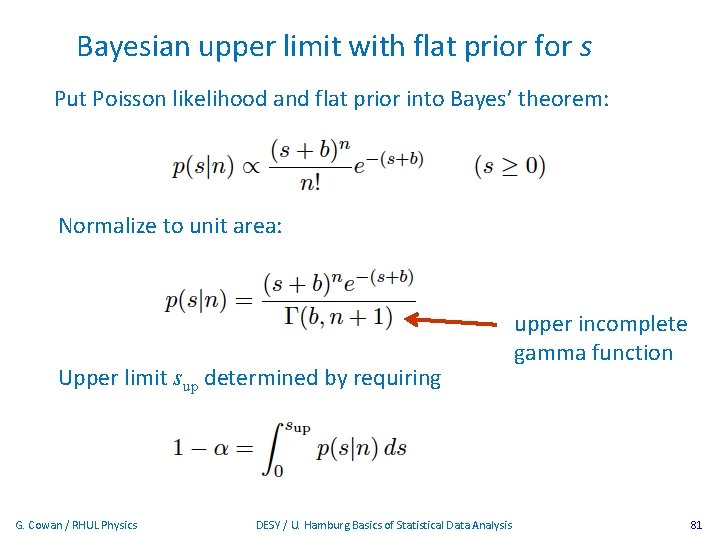
Bayesian upper limit with flat prior for s Put Poisson likelihood and flat prior into Bayes’ theorem: Normalize to unit area: Upper limit sup determined by requiring G. Cowan / RHUL Physics DESY / U. Hamburg Basics of Statistical Data Analysis upper incomplete gamma function 81

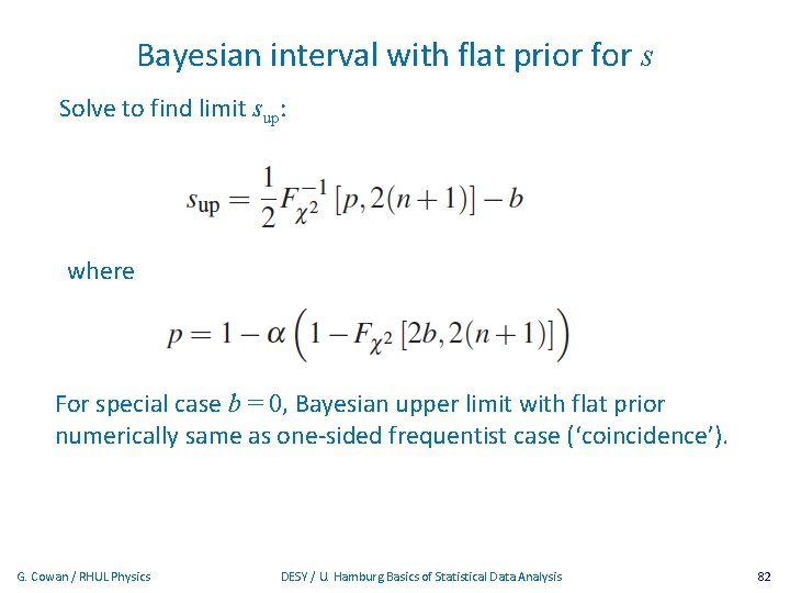
Bayesian interval with flat prior for s Solve to find limit sup: where For special case b = 0, Bayesian upper limit with flat prior numerically same as one-sided frequentist case (‘coincidence’). G. Cowan / RHUL Physics DESY / U. Hamburg Basics of Statistical Data Analysis 82

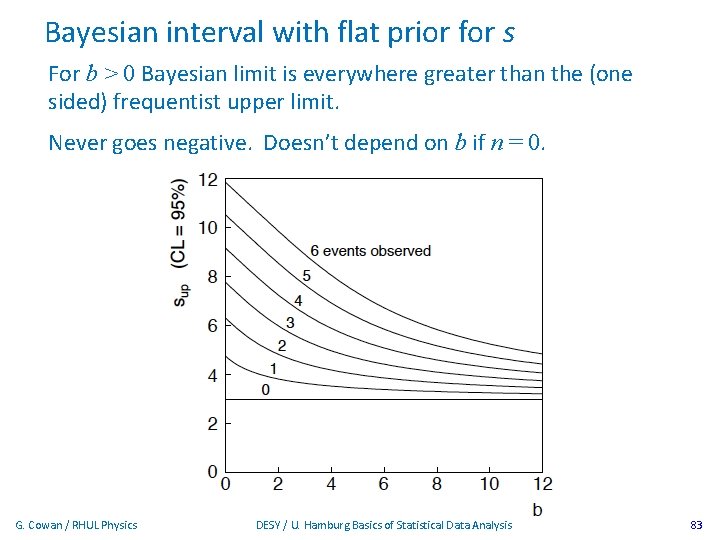
Bayesian interval with flat prior for s For b > 0 Bayesian limit is everywhere greater than the (one sided) frequentist upper limit. Never goes negative. Doesn’t depend on b if n = 0. G. Cowan / RHUL Physics DESY / U. Hamburg Basics of Statistical Data Analysis 83