Basics of demographic analysis 2 Life tables cohortcomponent
Basics of demographic analysis (2): Life tables, cohort-component projections Pia Wohland
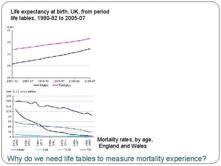
Life expectancy at birth, UK, from period life tables, 1980 -82 to 2005 -07 Mortality rates, by age, England Wales Why do we need life tables to measure mortality experience?
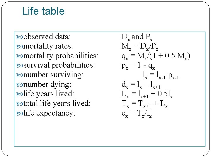
Life table observed data: mortality rates: mortality probabilities: survival probabilities: number surviving: number dying: life years lived: total life years lived: life expectancy: Dx and Px Mx = Dx/Px qx = Mx/(1 + 0. 5 Mx) px = 1 - qx lx = lx-1 px-1 dx = lx – lx+1 Lx = lx+1 + 0. 5 lx Tx = Tx+1 + Lx ex = Tx/lx
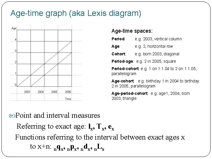
Age-time graph (aka Lexis diagram) Age-time spaces: Period: e. g. 2003, vertical column Age: e. g. 2, horizontal row Cohort: e. g. born 2003, diagonal Period-age: e. g. 2 in 2005, square Period-cohort: e. g. 1 on 1. 1. 04 to 2 on 1. 1. 05, parallelogram Age-cohort: e. g. birthday 1 in 2004 to birthday 2 in 2005, parallelogram Age-period-cohort: e. g. age 1, 2004, born 2003, triangle Point and interval measures Referring to exact age: lx, Tx, ex Functions referring to the interval between exact ages x to x+n: nqx, npx, ndx, n. Lx
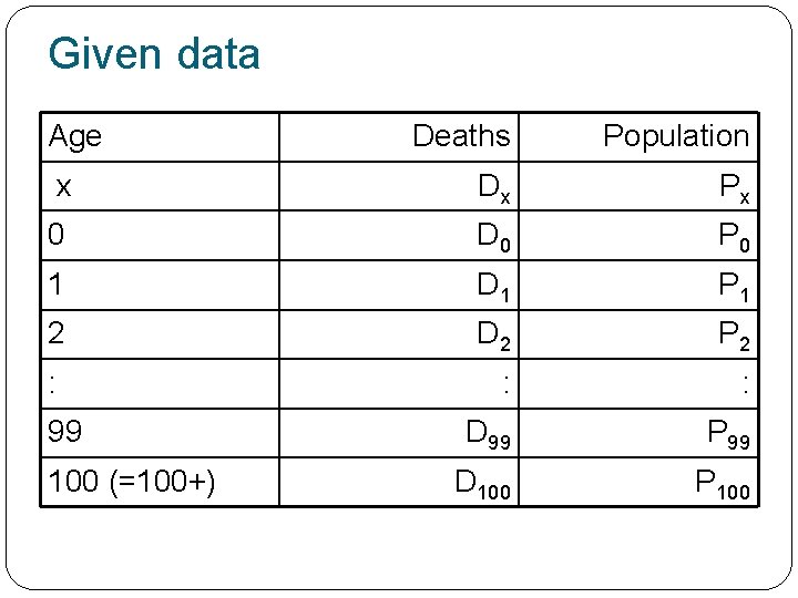
Given data Age Deaths Population x Dx Px 0 D 0 P 0 1 D 1 P 1 2 D 2 P 2 : : : D 99 P 99 D 100 P 100 99 100 (=100+)
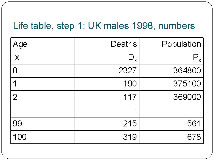
Life table, step 1: UK males 1998, numbers Age Deaths Population x Dx Px 0 2327 364800 1 190 375100 2 117 369000 : : : 99 215 561 100 319 678

Life table, step 2: compute observed mortality rates by age, Mx Mortality rate at age x = Deaths at age x/Population at risk at age x Deaths are recorded in period-age age-time spaces Population at risk either mid-year population aged x or average of start and end of year population aged x
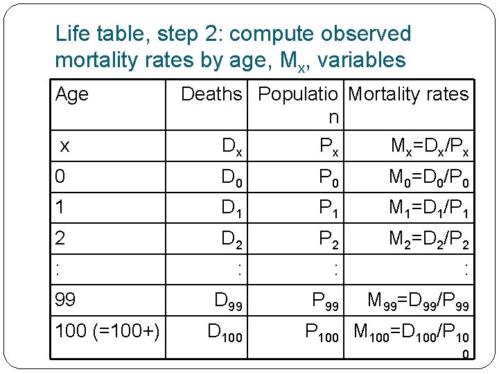
Life table, step 2: compute observed mortality rates by age, Mx, variables Age x Deaths Populatio Mortality rates n Dx Px Mx=Dx/Px 0 D 0 P 0 M 0=D 0/P 0 1 D 1 P 1 M 1=D 1/P 1 2 D 2 P 2 M 2=D 2/P 2 : : D 99 P 99 M 99=D 99/P 99 99 100 (=100+) D 100 P 100 M 100=D 100/P 10 0
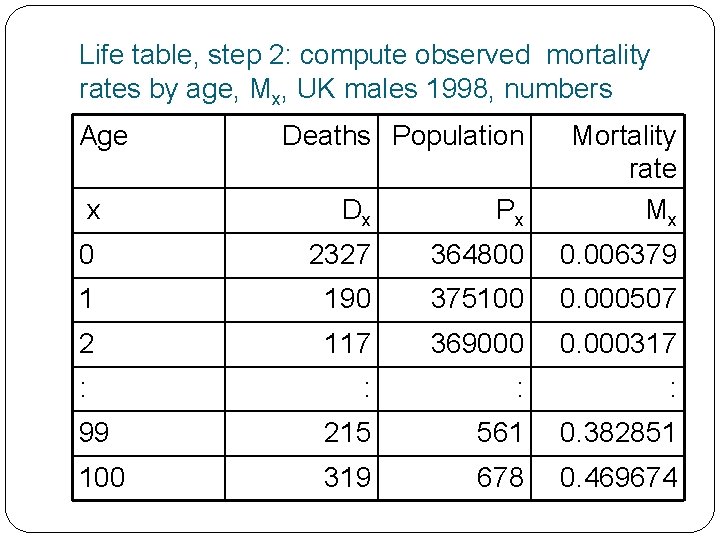
Life table, step 2: compute observed mortality rates by age, Mx, UK males 1998, numbers Age Deaths Population x Dx Px Mortality rate Mx 0 2327 364800 0. 006379 1 190 375100 0. 000507 2 117 369000 0. 000317 : : 99 215 561 0. 382851 100 319 678 0. 469674

Life table, step 3: compute the probabilities of dying between age x and x+1, qx The equation qx = Mx/(1 + 0. 5 Mx) sometimes given as qx = 2 Mx/(2 + Mx) Derivation Persons with xth birthday in year = Px + 0. 5 Dx Probability of dying between ages x and x+1 = Dx/(Px + 0. 5 Dx) Divide top and bottom by Px qx = (Dx/Px) / ([Px/Px] + 0. 5 [Dx/Px]) Substitute definition of Mx qx = Mx / (1 + 0. 5 Mx)
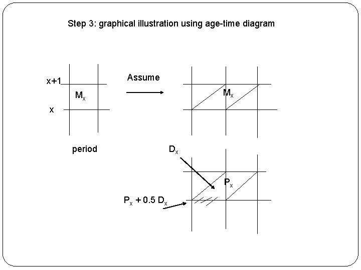
Step 3: graphical illustration using age-time diagram Assume x+1 Mx Mx x period Dx Px Px + 0. 5 Dx
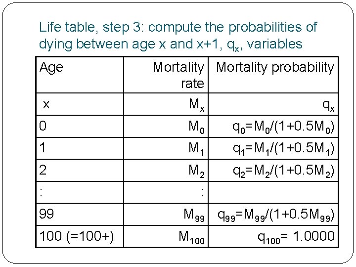
Life table, step 3: compute the probabilities of dying between age x and x+1, qx, variables Age x Mortality probability rate Mx qx 0 M 0 q 0=M 0/(1+0. 5 M 0) 1 M 1 q 1=M 1/(1+0. 5 M 1) 2 M 2 q 2=M 2/(1+0. 5 M 2) : : 99 100 (=100+) M 99 q 99=M 99/(1+0. 5 M 99) M 100 q 100= 1. 0000
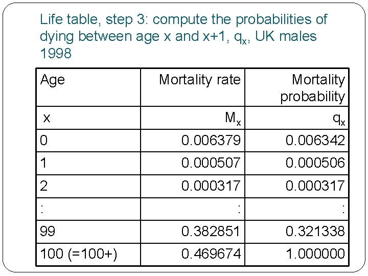
Life table, step 3: compute the probabilities of dying between age x and x+1, qx, UK males 1998 Age Mortality rate x Mx Mortality probability qx 0 0. 006379 0. 006342 1 0. 000507 0. 000506 2 0. 000317 : : : 99 0. 382851 0. 321338 100 (=100+) 0. 469674 1. 000000
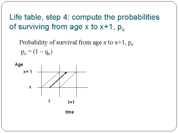
Life table, step 4: compute the probabilities of surviving from age x to x+1, px Probability of survival from age x to x+1, px px = (1 – qx) Age x+ 1 x t t+1 time
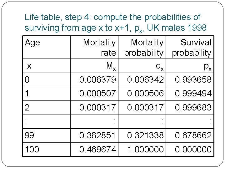
Life table, step 4: compute the probabilities of surviving from age x to x+1, px, UK males 1998 Age x Mortality Survival rate probability Mx qx px 0 0. 006379 0. 006342 0. 993658 1 0. 000507 0. 000506 0. 999494 2 0. 000317 0. 999683 : : 99 0. 382851 0. 321338 0. 678662 100 0. 469674 1. 000000 0. 000000

Life table, step 5: compute the numbers surviving to age x, lx - concept Life tables have a radix (number base) = hypothetical constant number born each year into a stationary population Usually radix = 100000 but you can use 10000 or 1000000 or 1 (in this case the survivors variable has a probability interpretation) lx = number of survivors of birth cohort who have attained age x (exact age or birthday) The number surviving to age x is the number surviving to age x-1 times the probability of surviving from age x-1 to age x
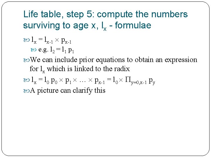
Life table, step 5: compute the numbers surviving to age x, lx - formulae lx = lx-1 px-1 e. g. l 2 = l 1 p 1 We can include prior equations to obtain an expression for lx which is linked to the radix lx = l 0 p 0 p 1 … px-1 = l 0 y=0, x-1 py A picture can clarify this

Surviving a birth cohort from one birthday to the next Age 4 3 l 3 p 2 2 l 2 p 1 1 l 1 p 0 0 l 0 t t+1 t+2 t+3 Time
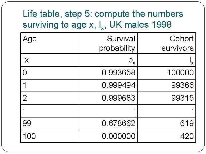
Life table, step 5: compute the numbers surviving to age x, lx, UK males 1998 Age x Survival probability px Cohort survivors lx 0 0. 993658 100000 1 0. 999494 99366 2 0. 999683 99315 : : : 99 0. 678662 619 100 0. 000000 420
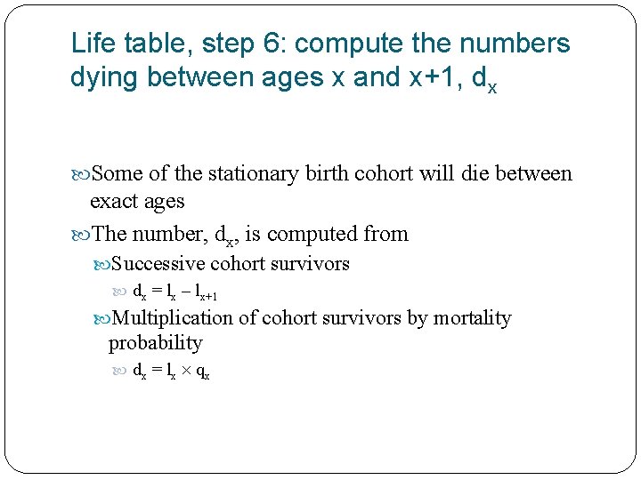
Life table, step 6: compute the numbers dying between ages x and x+1, dx Some of the stationary birth cohort will die between exact ages The number, dx, is computed from Successive cohort survivors dx = lx – lx+1 Multiplication of cohort survivors by mortality probability dx = lx qx
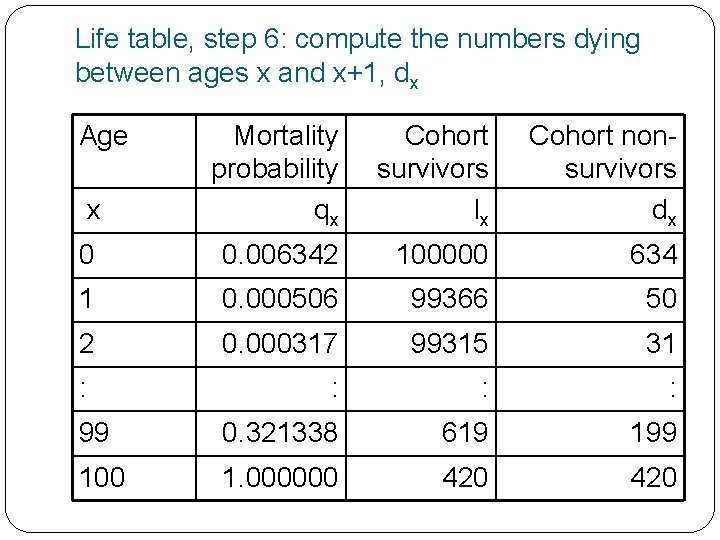
Life table, step 6: compute the numbers dying between ages x and x+1, dx Age x Mortality probability qx Cohort survivors lx Cohort nonsurvivors dx 0 0. 006342 100000 634 1 0. 000506 99366 50 2 0. 000317 99315 31 : : 99 0. 321338 619 199 100 1. 000000 420

Life table, step 8: compute the life years lived between ages x and x+1, Lx, concepts The next step is to work out how many years people in the birth cohort live between exact ages This quantity is called Lx and is made up of two parts, the life years lived by persons surviving through the interval and the life years lived by those who die in the interval We make an assumption about the fraction of the interval, called ax that non-survivors are alive for e. g. ax = 0. 5 for most ages (except the very young and oldest)
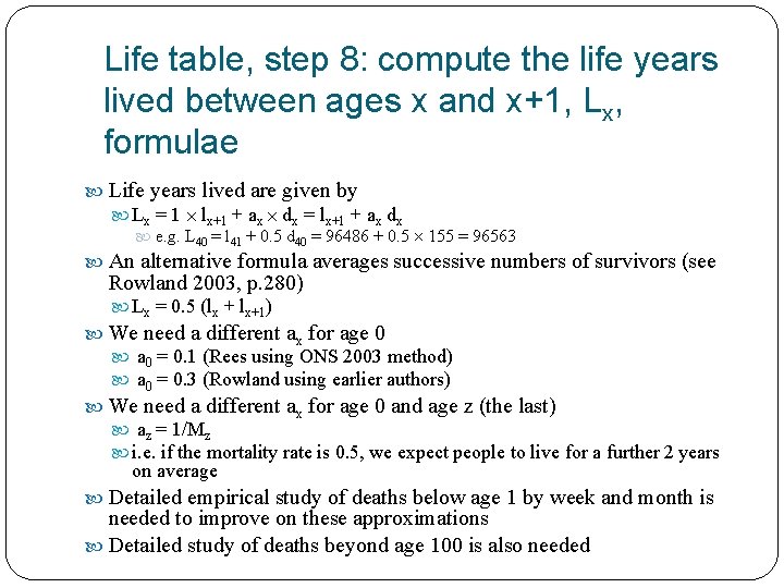
Life table, step 8: compute the life years lived between ages x and x+1, Lx, formulae Life years lived are given by Lx = 1 lx+1 + ax dx = lx+1 + ax dx e. g. L 40 = l 41 + 0. 5 d 40 = 96486 + 0. 5 155 = 96563 An alternative formula averages successive numbers of survivors (see Rowland 2003, p. 280) Lx = 0. 5 (lx + lx+1) We need a different ax for age 0 a 0 = 0. 1 (Rees using ONS 2003 method) a 0 = 0. 3 (Rowland using earlier authors) We need a different ax for age 0 and age z (the last) az = 1/Mz i. e. if the mortality rate is 0. 5, we expect people to live for a further 2 years on average Detailed empirical study of deaths below age 1 by week and month is needed to improve on these approximations Detailed study of deaths beyond age 100 is also needed

Illustration of the two meanings of Lx Age x+2 Lx+1 lx+1 Sx x+1 (2) Stationary population in age group Lx Lx (1) Life years lived between ages x lx t t+1 Time
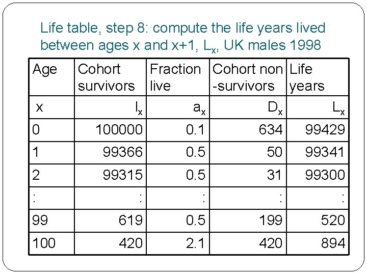
Life table, step 8: compute the life years lived between ages x and x+1, Lx, UK males 1998 Age x Cohort Fraction Cohort non Life survivors live -survivors years lx ax Dx Lx 0 100000 0. 1 634 99429 1 99366 0. 5 50 99341 2 99315 0. 5 31 99300 : : : 99 619 0. 5 199 520 100 420 2. 1 420 894
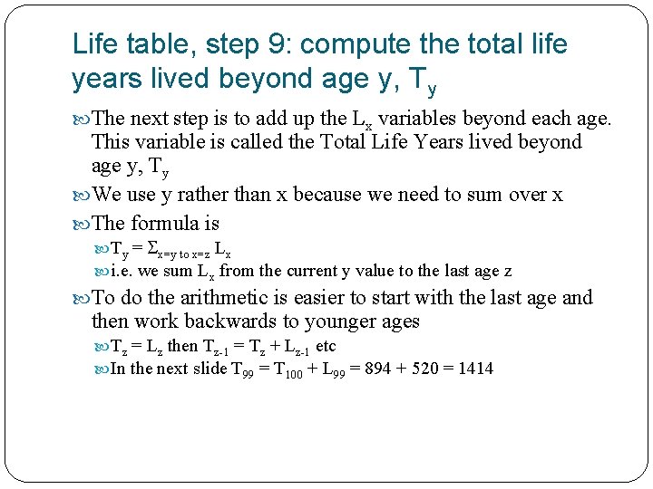
Life table, step 9: compute the total life years lived beyond age y, Ty The next step is to add up the Lx variables beyond each age. This variable is called the Total Life Years lived beyond age y, Ty We use y rather than x because we need to sum over x The formula is Ty = x=y to x=z Lx i. e. we sum Lx from the current y value to the last age z To do the arithmetic is easier to start with the last age and then work backwards to younger ages Tz = Lz then Tz-1 = Tz + Lz-1 etc In the next slide T 99 = T 100 + L 99 = 894 + 520 = 1414
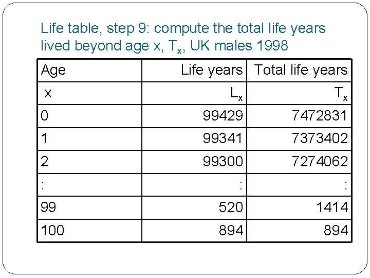
Life table, step 9: compute the total life years lived beyond age x, Tx, UK males 1998 Age Life years Total life years x Lx Tx 0 99429 7472831 1 99341 7373402 2 99300 7274062 : : : 99 520 1414 100 894
Life table, step 10: compute life expectancy beyond age x, ex The life expectancy at age x is the total number of life years lived beyond age x divided by the numbers in the birth cohort surviving to age x ex = T x / l x e. g. e 0 = T 0 / l 0 = life expectancy at birth Also of interest are e 65, e 70, e 75, e 80 for pension, health care and personal care planning for the older population
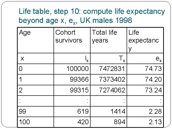
Life table, step 10: compute life expectancy beyond age x, ex, UK males 1998 Age Cohort survivors Total life years Life expectanc y Tx ex x lx 0 100000 7472831 74. 73 1 99366 7373402 74. 20 2 99315 7274062 73. 24 : : 99 619 1414 2. 28 100 420 894 2. 13
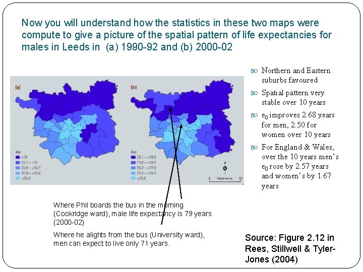
Now you will understand how the statistics in these two maps were compute to give a picture of the spatial pattern of life expectancies for males in Leeds in (a) 1990 -92 and (b) 2000 -02 Northern and Eastern suburbs favoured Spatial pattern very stable over 10 years e 0 improves 2. 68 years for men, 2. 50 for women over 10 years For England & Wales, over the 10 years men’s e 0 rose by 2. 57 years and women’s by 1. 67 years Where Phil boards the bus in the morning (Cookridge ward), male life expectancy is 79 years (2000 -02) Where he alights from the bus (University ward), men can expect to live only 71 years. Source: Figure 2. 12 in Rees, Stillwell & Tyler. Jones (2004)
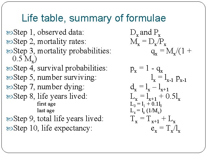
Life table, summary of formulae Step 1, observed data: Step 2, mortality rates: Step 3, mortality probabilities: 0. 5 Mx) Step 4, survival probabilities: Step 5, number surviving: Step 7, number dying: Step 8, life years lived: first age last age Step 9, total life years lived: Step 10, life expectancy: Dx and Px Mx = Dx/Px qx = Mx/(1 + px = 1 - qx lx = lx-1 px-1 dx = lx – lx+1 Lx = lx+1 + 0. 5 lx L 0 = l 1 + 0. 1 l 0 Lz = lz (1/Mz) Tx = Tx+1 + Lx ex = Tx/lx
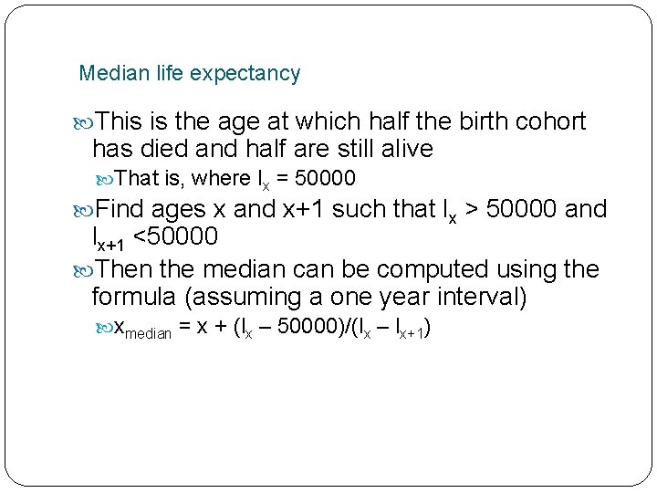
Median life expectancy This is the age at which half the birth cohort has died and half are still alive That is, where lx = 50000 Find ages x and x+1 such that lx > 50000 and lx+1 <50000 Then the median can be computed using the formula (assuming a one year interval) xmedian = x + (lx – 50000)/(lx – lx+1)
Cohort component projection

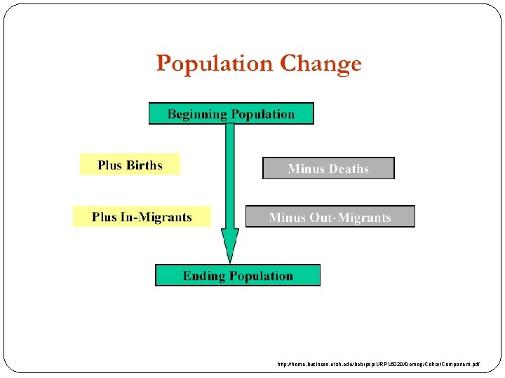
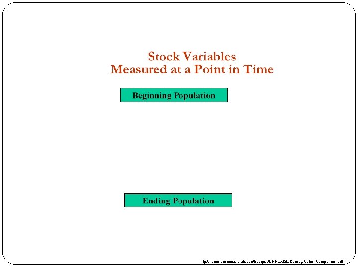
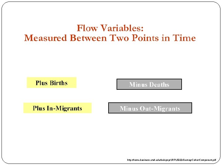
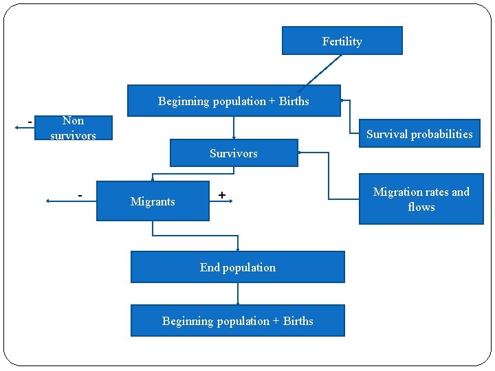
Cohort Component Model Type of population projection model Separately accounts for 3 components of population change: • Births • Deaths • Migration +Age, sex, geographic, ethnicity The model is used to account for population change.
http: //home. business. utah. edu/bebrpsp/URPL 5020/Demog/Cohort. Component. pdf
http: //home. business. utah. edu/bebrpsp/URPL 5020/Demog/Cohort. Component. pdf
http: //home. business. utah. edu/bebrpsp/URPL 5020/Demog/Cohort. Component. pdf
Fertility Beginning population + Births - Non survivors Survival probabilities Survivors - Migrants + End population Beginning population + Births Migration rates and flows
The cohort-component projection model Components of population change: Population next year = Population last year minus Deaths plus Births plus Net Migration Cohort Each component needs to be decomposed by age Births are introduced into the first age group Deaths cluster in older ages Migration is highest in the young adult ages Fertility is age dependent Cohort-component intensities are used Survival probabilities (the complement of mortality probabilities) Fertility rates (occurrence-exposure) by age of mother Net migration counts by age The C-C model normally uses both sexes
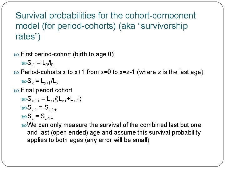
Survival probabilities for the cohort-component model (for period-cohorts) (aka “survivorship rates”) First period-cohort (birth to age 0) S-1 = L 0/l 0 Period-cohorts x to x+1 from x=0 to x=z-1 (where z is the last age) Sx = Lx+1/Lx Final period cohort Sz-1+ = Lz+/(Lz++Lz-1) Sz-1 = Sz-1+ Sz = Sz-1+ We can only measure the survival of the combined last but one and last (open ended) age and assume this survival probability applies to both ages (any error will be small)

age First period-cohort Standard period-cohort x+2 L 0 Lx+1 S-1 0 x+1 l 0 x+1 Lx time x -1 Lz t t+1 Lz z Last but one and last period-cohorts Lz-1 t t+1

The cohort-component model (1) Notation P = population s = survival probability N = net migration B = births x = age (usually period-cohort) z = last age (open ended), z-1 = last but one age, -1 = birth g = gender with values m (males) and f (females) t = time point (start of interval) w = sex probability (at birth) We need three sets of equations for The “infant” period-cohort, birth to age 0 The standard period-cohorts, from age 0 to age z-1 The last period-cohort, from age z+ to age z+
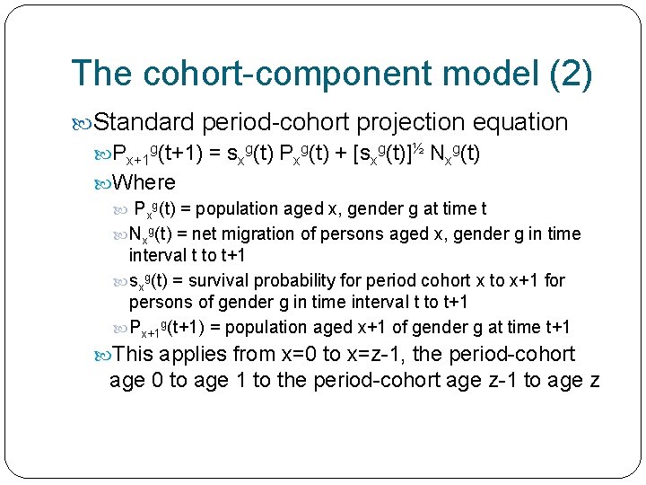
The cohort-component model (2) Standard period-cohort projection equation Px+1 g(t+1) = sxg(t) Pxg(t) + [sxg(t)]½ Nxg(t) Where Pxg(t) = population aged x, gender g at time t Nxg(t) = net migration of persons aged x, gender g in time interval t to t+1 sxg(t) = survival probability for period cohort x to x+1 for persons of gender g in time interval t to t+1 Px+1 g(t+1) = population aged x+1 of gender g at time t+1 This applies from x=0 to x=z-1, the period-cohort age 0 to age 1 to the period-cohort age z-1 to age z

The cohort-component model (3) Last period-cohort projection equation Pzg(t+1) = sz-1 g(t) Pz-1 g(t) + [sz-1 g(t)]½ Nz-1 g(t) + szg(t) Pzg(t) + [szg(t)]½ Nzg(t) We survive persons aged z-1 into z and add persons surviving within z, the last open ended age group e. g. 100 + = survivors from 99 to 100 plus from 100+ to 100+
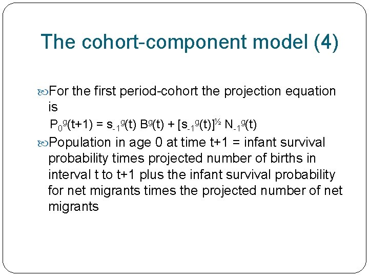
The cohort-component model (4) For the first period-cohort the projection equation is P 0 g(t+1) = s-1 g(t) Bg(t) + [s-1 g(t)]½ N-1 g(t) Population in age 0 at time t+1 = infant survival probability times projected number of births in interval t to t+1 plus the infant survival probability for net migrants times the projected number of net migrants
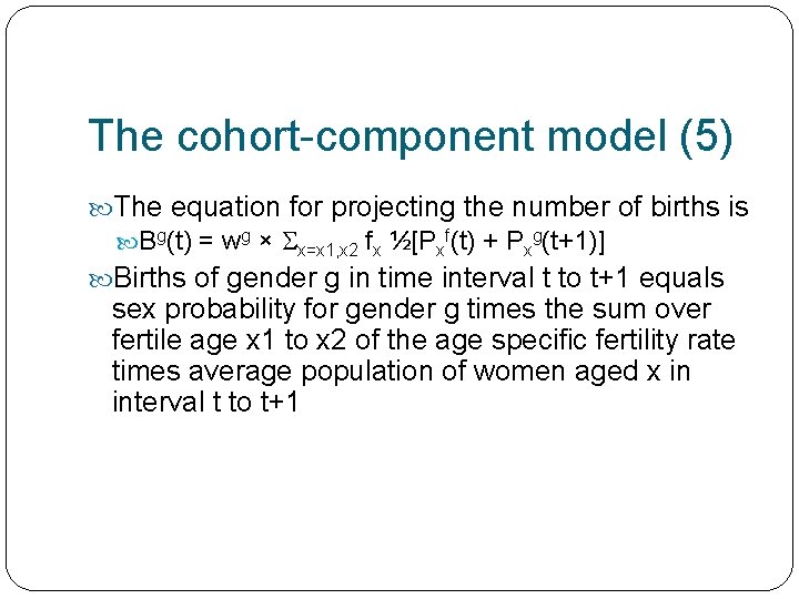
The cohort-component model (5) The equation for projecting the number of births is Bg(t) = wg × x=x 1, x 2 fx ½[Pxf(t) + Pxg(t+1)] Births of gender g in time interval t to t+1 equals sex probability for gender g times the sum over fertile age x 1 to x 2 of the age specific fertility rate times average population of women aged x in interval t to t+1

More to consider: changes over time migration new births/fertility survival
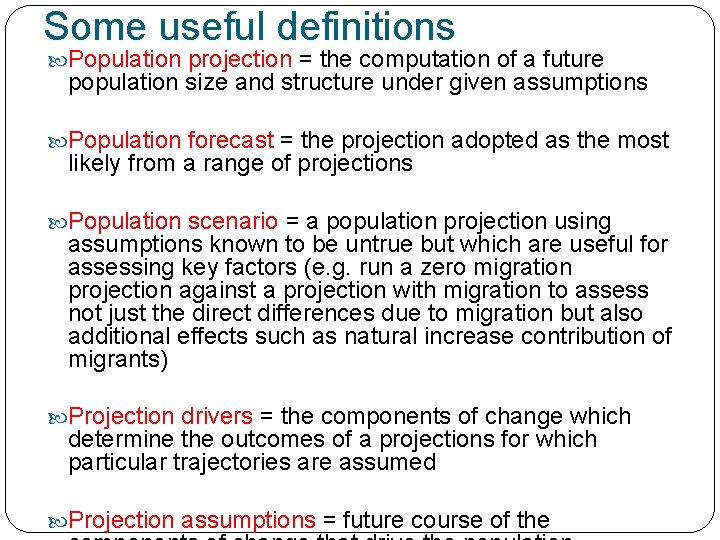
Some useful definitions Population projection = the computation of a future population size and structure under given assumptions Population forecast = the projection adopted as the most likely from a range of projections Population scenario = a population projection using assumptions known to be untrue but which are useful for assessing key factors (e. g. run a zero migration projection against a projection with migration to assess not just the direct differences due to migration but also additional effects such as natural increase contribution of migrants) Projection drivers = the components of change which determine the outcomes of a projections for which particular trajectories are assumed Projection assumptions = future course of the

- Slides: 49