Basic Statistics for Scientific Research Statistics involves math

Basic Statistics for Scientific Research

Statistics involves math and calculations of numbers. It also guides how numbers are chosen, interpreted, and compared to other numbers. Consider the following three scenarios and the interpretations based upon the presented statistics. You will find that the numbers may be right, but the interpretation may be wrong. Try to identify a major flaw with each interpretation before we describe it. 1) A new advertisement for Ben and Jerry's ice cream introduced in late May of last year resulted in a 30% increase in ice cream sales for the following three months. Thus, the advertisement was effective. A major flaw is that other things also affect ice cream consumption and these other variables were not controlled or accounted for. Ice cream consumption generally increases in the months of June, July, and August regardless of advertisements. This effect is called a history effect and leads people to interpret outcomes as the result of one variable when another variable (in this case, the passage of time) is actually responsible.

Statistics involves math and calculations of numbers. It also guides how numbers are chosen, interpreted, and compared to other numbers. Consider the following three scenarios and the interpretations based upon the presented statistics. You will find that the numbers may be right, but the interpretation may be wrong. Try to identify a major flaw with each interpretation before we describe it. 2) The more churches in a city, the more crime there is. Thus, churches lead to crime. A major flaw is that other things also affect crime rates and these other variables were not controlled or accounted for. Both increased churches and increased crime rates can be explained by larger populations. In bigger cities, there are both more churches and more crime. This problem is an eg of the thirdvariable problem. Namely, a third variable can cause both situations; however, people erroneously believe that there is a causal relationship between the two primary variables rather than recognize that a third variable can cause both.

Statistics involves math and calculations of numbers. It also guides how numbers are chosen, interpreted, and compared to other numbers. Consider the following three scenarios and the interpretations based upon the presented statistics. You will find that the numbers may be right, but the interpretation may be wrong. Try to identify a major flaw with each interpretation before we describe it. 3) You measured the fall time of an object repeatedly and experimentally determined the acceleration due to gravity to be 9. 3 m/s 2. Does your result agree with the accepted value of 9. 8 m/s 2? NO MEASUREMENT IS EXACT because there are random errors in every measurement. Therefore, every measured value really represents a range of values (9. 3 ± uncertainty). Without knowledge of the uncertainty in the average value, no comparison between the 2 results can be made. How close is close enough for agreement?

Statistics is not just mathematics and calculations of numbers. It is also a guide to interpreting those numbers.

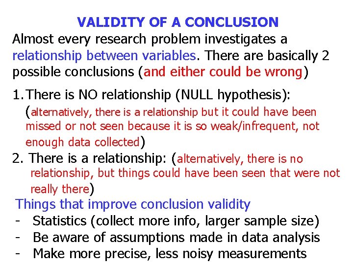
VALIDITY OF A CONCLUSION Almost every research problem investigates a relationship between variables. There are basically 2 possible conclusions (and either could be wrong) 1. There is NO relationship (NULL hypothesis): (alternatively, there is a relationship but it could have been missed or not seen because it is so weak/infrequent, not enough data collected) 2. There is a relationship: (alternatively, there is no relationship, but things could have been seen that were not really there) Things that improve conclusion validity - Statistics (collect more info, larger sample size) - Be aware of assumptions made in data analysis - Make more precise, less noisy measurements

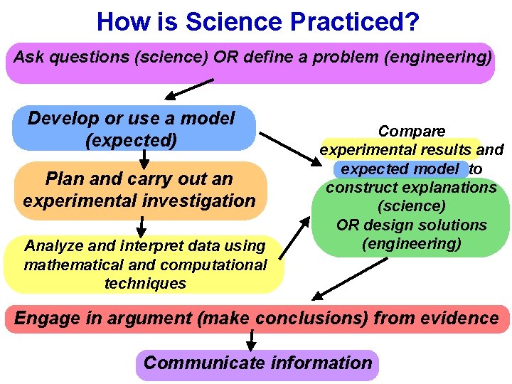
How is Science Practiced? Ask questions (science) OR define a problem (engineering) Develop or use a model (expected) Plan and carry out an experimental investigation Analyze and interpret data using mathematical and computational techniques Compare experimental results and expected model to construct explanations (science) OR design solutions (engineering) Engage in argument (make conclusions) from evidence Communicate information

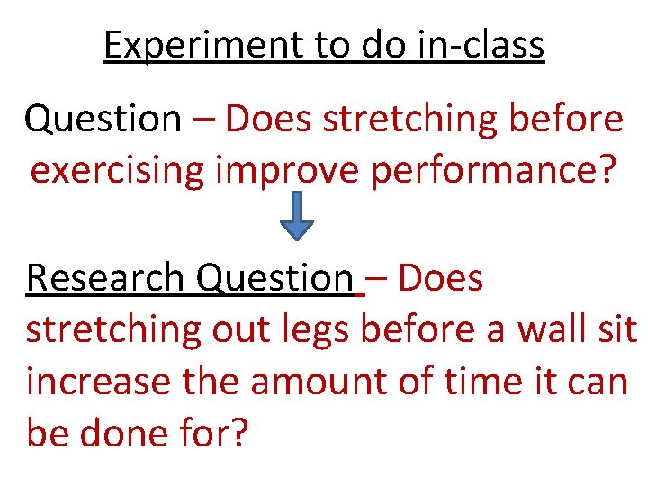
Experiment to do in-class Question – Does stretching before exercising improve performance? Research Question – Does stretching out legs before a wall sit increase the amount of time it can be done for?

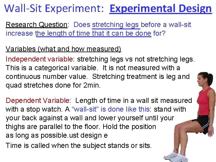
Wall-Sit Experiment: Experimental Design Research Question: Does stretching legs before a wall-sit increase the length of time that it can be done for? Variables (what and how measured) Independent variable: stretching legs vs not stretching legs. This is a categorical variable. It is not measured with a continuous number value. Stretching treatment is leg and quad stretches done for 2 min. Dependent Variable: Length of time in a wall sit measured with a stop watch. A “wall-sit” is done like this: stand with your back against a wall and lower yourself until your thighs are parallel to the floor. Hold the position as long as possible. ust design e Time is called when the subject stands or sits.

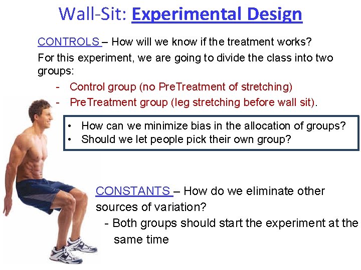
Wall-Sit: Experimental Design CONTROLS – How will we know if the treatment works? For this experiment, we are going to divide the class into two groups: - Control group (no Pre. Treatment of stretching) - Pre. Treatment group (leg stretching before wall sit). • How can we minimize bias in the allocation of groups? • Should we let people pick their own group? CONSTANTS – How do we eliminate other sources of variation? - Both groups should start the experiment at the same time

Wall-Sit Experiment: Analysis Research Question: Does stretching legs before a wallsit increase the length of time that it can be done for? http: //www. timeanddate. com/stopwatch • How could we display the data? • How can we quantify the effect of the treatment?

Descriptive Statistics Descriptive statistics can be used to summarize and describe a single variable at a time (UNIvariate analysis). There are 3 major characteristics of a single variable (found by repeating the measurement) 1. The distribution (frequencies, percentages) 2. The central tendency (mean, median) 3. The dispersion or spread around the central tendency (standard deviation, range)

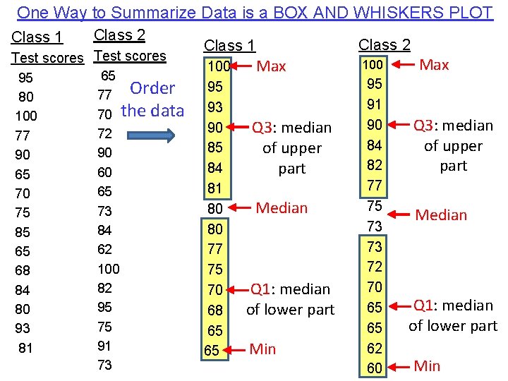
One Way to Summarize Data is a BOX AND WHISKERS PLOT Class 1 Class 2 Test scores 95 80 100 77 90 65 70 75 85 65 68 84 80 93 81 65 77 Order 70 the data 72 90 60 65 73 84 62 100 82 95 75 91 73 Class 2 Class 1 100 95 93 90 85 84 81 80 80 77 75 70 68 65 65 Max Q 3: median of upper part Median Q 1: median of lower part Min 100 95 91 90 84 82 77 75 73 73 72 70 65 65 62 60 Max Q 3: median of upper part Median Q 1: median of lower part Min

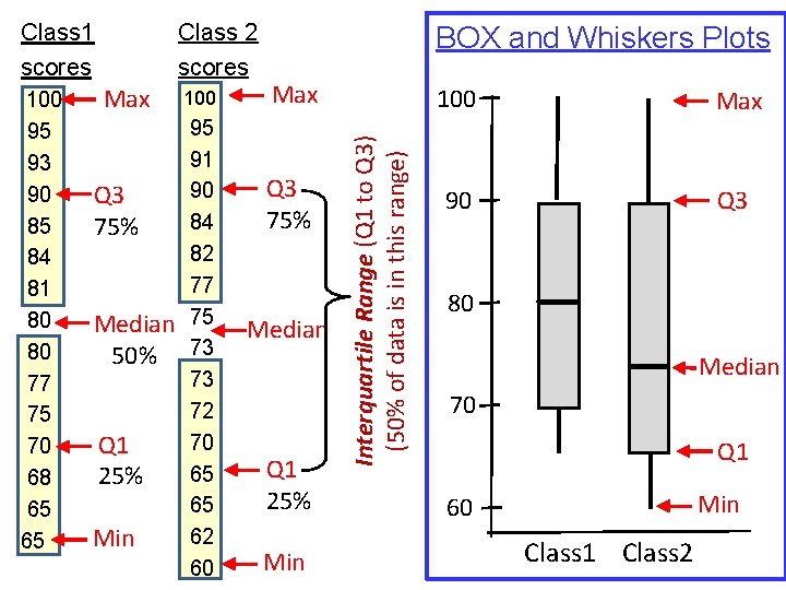
100 95 93 90 85 84 81 80 80 77 75 70 68 65 65 Max Q 3 75% Median 50% Q 1 25% Min 100 95 91 90 84 82 77 75 73 73 72 70 65 65 62 60 BOX and Whiskers Plots Max Q 3 75% Median Q 1 25% Min Interquartile Range (Q 1 to Q 3) (50% of data is in this range) Class 2 scores Class 1 scores 100 Max 90 Q 3 80 Median 70 Q 1 Min 60 Class 1 Class 2

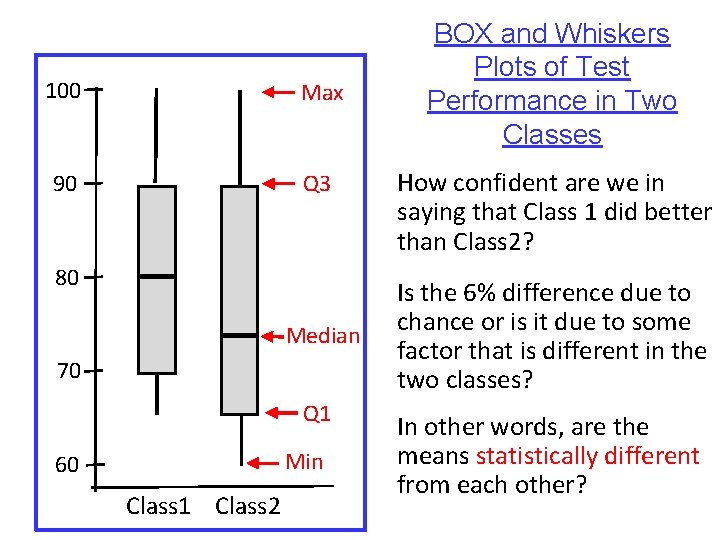
100 Max 90 Q 3 80 Median 70 Q 1 Min 60 Class 1 Class 2 BOX and Whiskers Plots of Test Performance in Two Classes How confident are we in saying that Class 1 did better than Class 2? Is the 6% difference due to chance or is it due to some factor that is different in the two classes? In other words, are the means statistically different from each other?

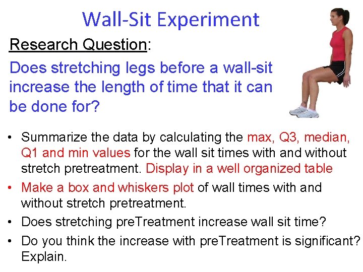
Wall-Sit Experiment Research Question: Does stretching legs before a wall-sit increase the length of time that it can be done for? • Summarize the data by calculating the max, Q 3, median, Q 1 and min values for the wall sit times with and without stretch pretreatment. Display in a well organized table • Make a box and whiskers plot of wall times with and without stretch pretreatment. • Does stretching pre. Treatment increase wall sit time? • Do you think the increase with pre. Treatment is significant? Explain.

In most research, data analysis involves three major steps, done in roughly this order: • Data Preparation - Logging, cleaning and organizing the data for analysis • Descriptive Statistics – numbers used to summarize and describe data. Together with graphical analysis, they form the basis of almost every quantitative analysis of data. With descriptive stats, you are simply describing what the data shows • Inferential Statistics - Testing Hypotheses and Models. Conclusions from inferential stats extends beyond the immediate data (sample) and tries to infer more general conclusions (population)

Types of Statistics/Analyses Descriptive Statistics – describes basic features of data. Simplifies large amounts of data with single indicators How many? How much? – Means (central tendency) How variable? How – standard deviation/variance uncertain? (dispersion around mean) BP, HR, BMI, IQ, etc. – Frequencies/percentages (distribution) Inferential Statistics – goes beyond the immediate data to make inferences about population phenomena – – – Hypothesis Testing Correlation Confidence Intervals / T-tests Significance Testing Prediction Proving or disproving theories Associations between phenomena If sample relates to the larger population E. g. , Diet and health

Descriptive Statistics used to present quantitative descriptions in a manageable form. In a research study there may be lots of measures. Descriptive statistics helps simplify large amounts of data in a sensible way. Each descriptive statistic reduces lots of data into a simpler summary. Using a single indicator for Examples of Descriptive Stats a large set of observations can distort the original data or loose important detail - Batting average –summarizes how well batter performs. The single number describes a large number of discrete events. doesn’t tell whether hits are HRs or singles, whether slump or streak. - Grade Point Average (GPA)-single doesn’t tell whether difficult or easy courses, major field number that describes the general performance of a student or others across a potentially wide range of course experiences.

Descriptive Statistics Descriptive statistics can be used to summarize and describe a single variable at a time (UNIvariate analysis). There are 3 major characteristics of a single variable (found by repeating the measurement) 1. The distribution (frequencies, percentages) 2. The central tendency (mean, median, mode) 3. The dispersion or spread around the central tendency (standard deviation, range)

Types of Variables QUANTITATIVE CONTINUOUS or QUALITATIVE DISCRETE or TYPE DEFINITION EXAMPLES Categorical Variable that can take on one of a or nominal limited number of possible values, groups or categories. There is no intrinsic ordering to the categories. Gender haircolor Bloodtype (A, B, AB, O) State resident lives in Ordinal Similar to categorical, but there is a clear ordering of the variables Economic class Interval Similar to ordinal except the intervals between the values of the interval variable are equally spaced so they can be measured along a continuum and given numerical values Annual income Temperature Reaction time BP Ratio interval variables, but with the added condition that 0 of the measurement indicates that there is none of that variable. You can use ratios to relate these measurements. Height Mass Distance weight Temp only in Kelvin Educational experience Likert scales or ratings

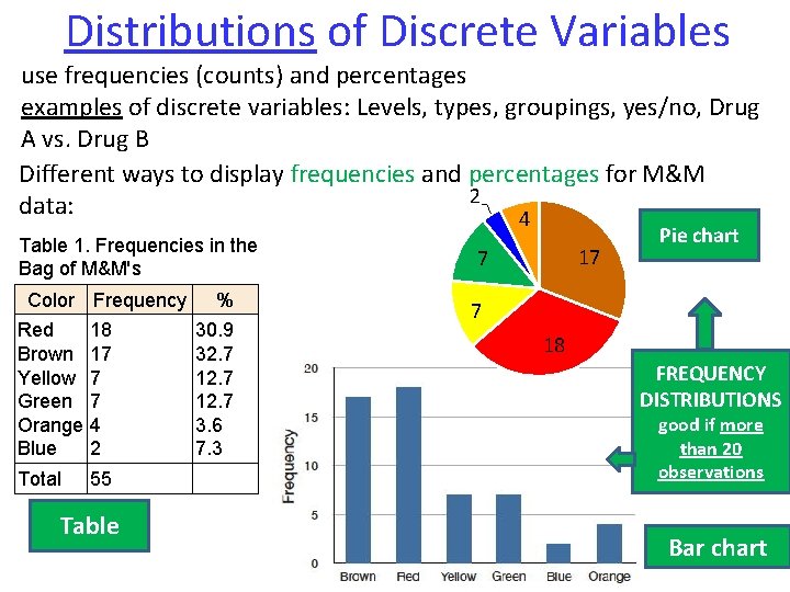
Distributions of Discrete Variables use frequencies (counts) and percentages examples of discrete variables: Levels, types, groupings, yes/no, Drug A vs. Drug B Different ways to display frequencies and percentages for M&M 2 data: 4 Table 1. Frequencies in the Bag of M&M's Color Frequency Red Brown Yellow Green Orange Blue 18 17 7 7 4 2 Total 55 Table % 30. 9 32. 7 12. 7 3. 6 7. 3 17 7 Pie chart 7 18 FREQUENCY DISTRIBUTIONS good if more than 20 observations Bar chart

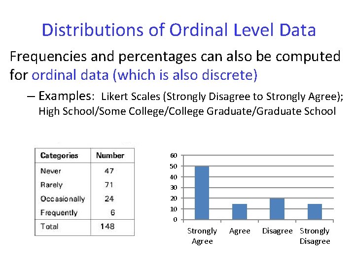
Distributions of Ordinal Level Data Frequencies and percentages can also be computed for ordinal data (which is also discrete) – Examples: Likert Scales (Strongly Disagree to Strongly Agree); High School/Some College/College Graduate/Graduate School 60 50 40 30 20 10 0 Strongly Agree Disagree Strongly Disagree

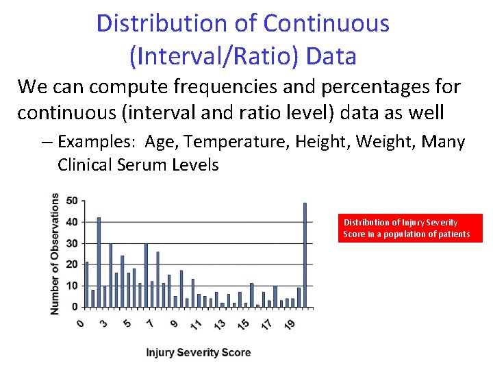
Distribution of Continuous (Interval/Ratio) Data We can compute frequencies and percentages for continuous (interval and ratio level) data as well – Examples: Age, Temperature, Height, Weight, Many Clinical Serum Levels Distribution of Injury Severity Score in a population of patients

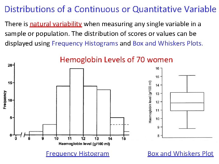
Distributions of a Continuous or Quantitative Variable There is natural variability when measuring any single variable in a sample or population. The distribution of scores or values can be displayed using Frequency Histograms and Box and Whiskers Plots. Hemoglobin Levels of 70 women Frequency Histogram Box and Whiskers Plot

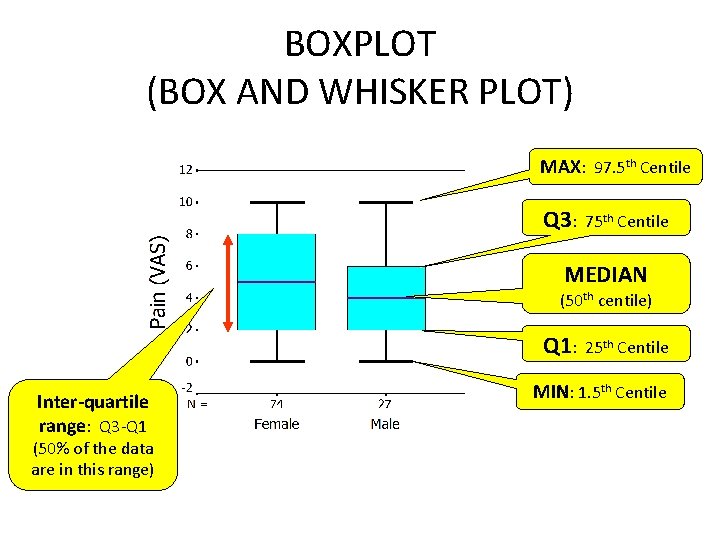
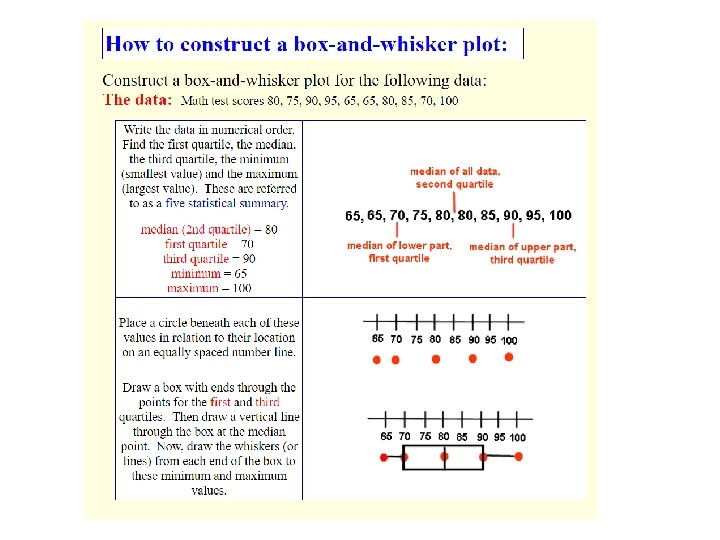
BOXPLOT (BOX AND WHISKER PLOT) MAX: 97. 5 th Centile Q 3: 75 th Centile MEDIAN (50 th centile) Q 1: 25 th Centile Inter-quartile range: Q 3 -Q 1 (50% of the data are in this range) MIN: 1. 5 th Centile

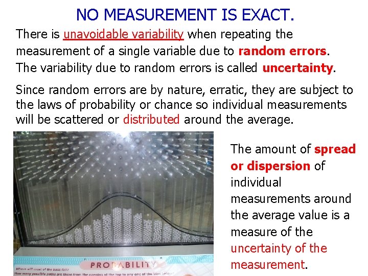
NO MEASUREMENT IS EXACT. There is unavoidable variability when repeating the measurement of a single variable due to random errors. The variability due to random errors is called uncertainty. Since random errors are by nature, erratic, they are subject to the laws of probability or chance so individual measurements will be scattered or distributed around the average. The amount of spread or dispersion of individual measurements around the average value is a measure of the uncertainty of the measurement.

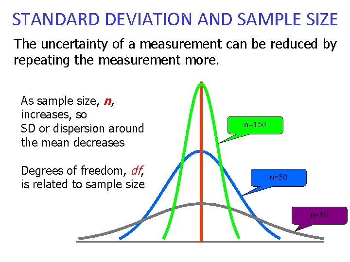
STANDARD DEVIATION AND SAMPLE SIZE The uncertainty of a measurement can be reduced by repeating the measurement more. As sample size, n, increases, so SD or dispersion around the mean decreases Degrees of freedom, df, is related to sample size n=150 n=10

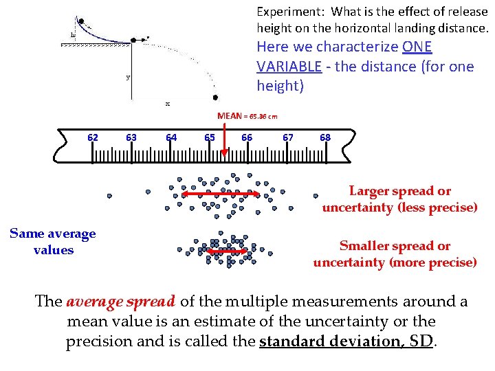
Experiment: What is the effect of release height on the horizontal landing distance. Here we characterize ONE VARIABLE - the distance (for one height) MEAN = 65. 36 cm 62 63 64 65 66 67 68 Larger spread or uncertainty (less precise) Same average values Smaller spread or uncertainty (more precise) The average spread of the multiple measurements around a mean value is an estimate of the uncertainty or the precision and is called the standard deviation, SD.

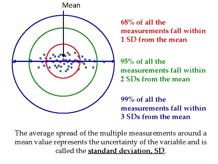
Mean 68% of all the measurements fall within 1 SD from the mean 95% of all the measurements fall within 2 SDs from the mean 99% of all the measurements fall within 3 SDs from the mean The average spread of the multiple measurements around a mean value represents the uncertainty of the variable and is called the standard deviation, SD.

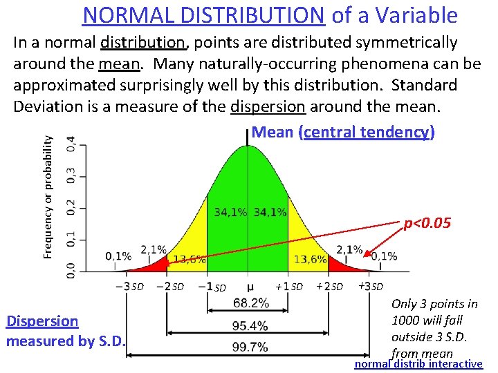
NORMAL DISTRIBUTION of a Variable Frequency or probability In a normal distribution, points are distributed symmetrically around the mean. Many naturally-occurring phenomena can be approximated surprisingly well by this distribution. Standard Deviation is a measure of the dispersion around the mean. Mean (central tendency) p<0. 05 SD Dispersion measured by S. D. SD SD + SD Only 3 points in 1000 will fall outside 3 S. D. from mean normal distrib interactive

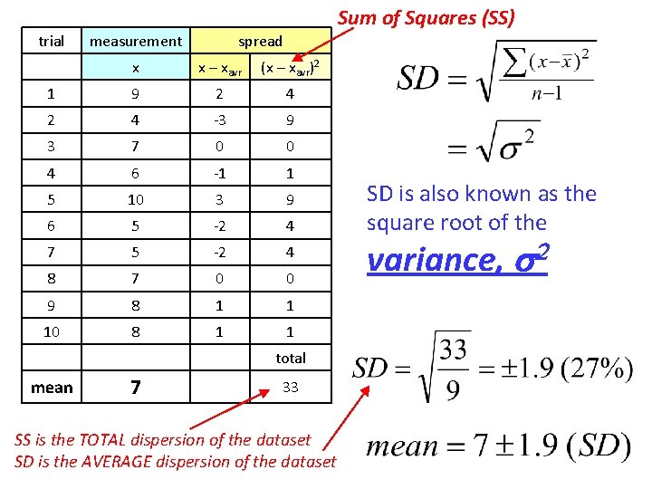
trial measurement Sum of Squares (SS) spread x x – xavr (x – xavr)2 1 9 2 4 -3 9 3 7 0 0 4 6 -1 1 5 10 3 9 6 5 -2 4 7 5 -2 4 8 7 0 0 9 8 1 1 10 8 1 1 total mean 7 33 SS is the TOTAL dispersion of the dataset SD is the AVERAGE dispersion of the dataset SD is also known as the square root of the variance, s 2

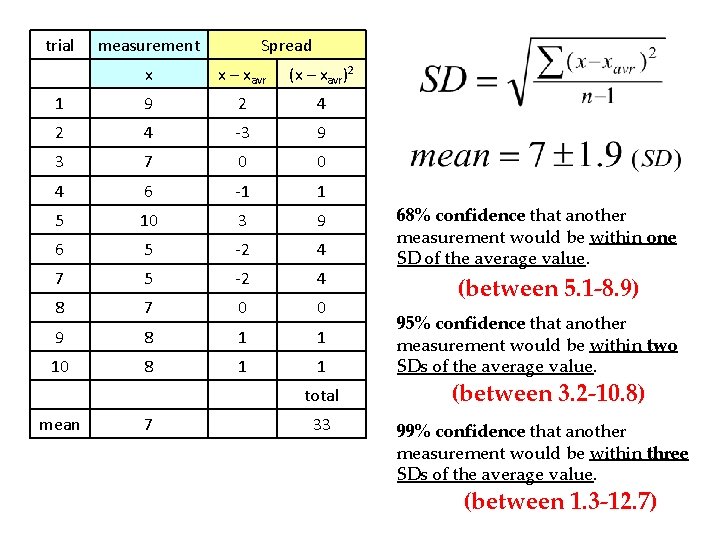
trial measurement Spread x x – xavr (x – xavr)2 1 9 2 4 -3 9 3 7 0 0 4 6 -1 1 5 10 3 9 6 5 -2 4 7 5 -2 4 8 7 0 0 9 8 1 1 10 8 1 1 total mean 7 33 68% confidence that another measurement would be within one SD of the average value. (between 5. 1 -8. 9) 95% confidence that another measurement would be within two SDs of the average value. (between 3. 2 -10. 8) 99% confidence that another measurement would be within three SDs of the average value. (between 1. 3 -12. 7)

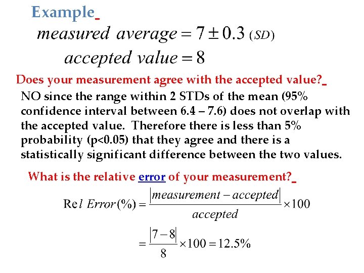
Example Does your measurement agree with the accepted value? NO since the range within 2 STDs of the mean (95% confidence interval between 6. 4 – 7. 6) does not overlap with the accepted value. Therefore there is less than 5% probability (p<0. 05) that they agree and there is a statistically significant difference between the two values. What is the relative error of your measurement?

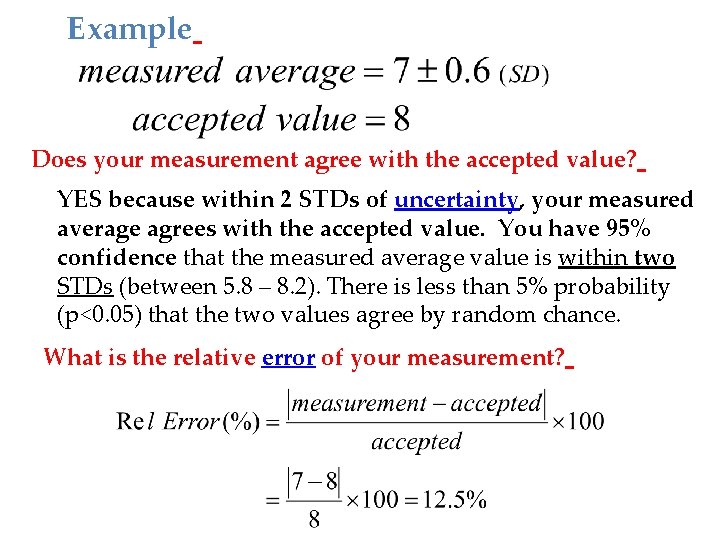
Example Does your measurement agree with the accepted value? YES because within 2 STDs of uncertainty, your measured average agrees with the accepted value. You have 95% confidence that the measured average value is within two STDs (between 5. 8 – 8. 2). There is less than 5% probability (p<0. 05) that the two values agree by random chance. What is the relative error of your measurement?

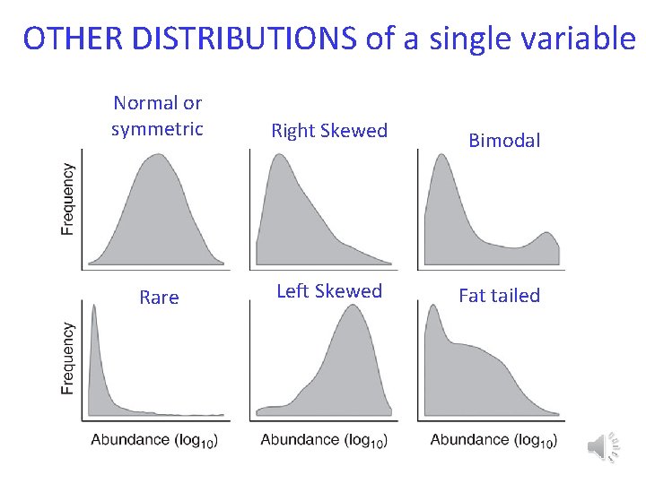
OTHER DISTRIBUTIONS of a single variable Normal or symmetric Right Skewed Bimodal Rare Left Skewed Fat tailed

DESCRIBING DATA – Central Tendency MEAN Average or arithmetic mean of the data MEDIAN The value which comes half way when the data are ranked in order MODE Most common value observed • In a normal distribution, mean and median are the same • If median and mean are different, indicates that the data are not normally distributed • The mode is of little if any practical use

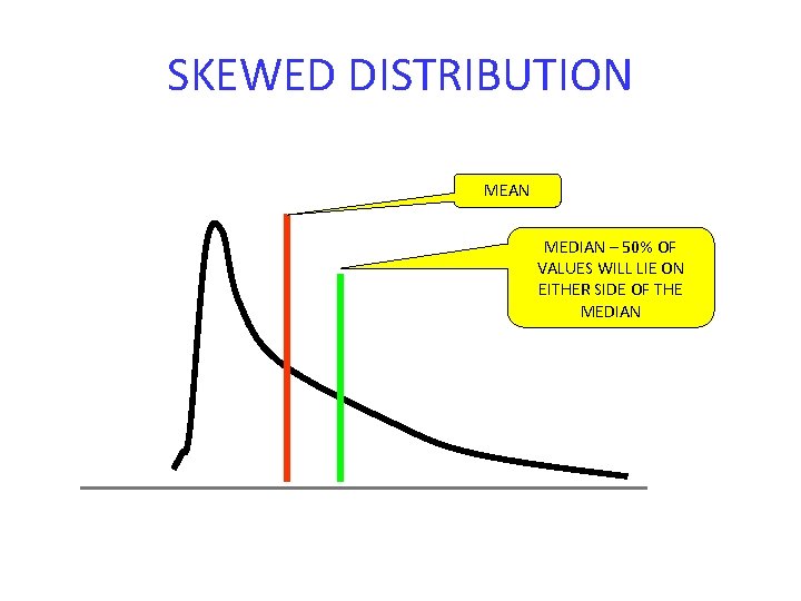
SKEWED DISTRIBUTION MEAN MEDIAN – 50% OF VALUES WILL LIE ON EITHER SIDE OF THE MEDIAN

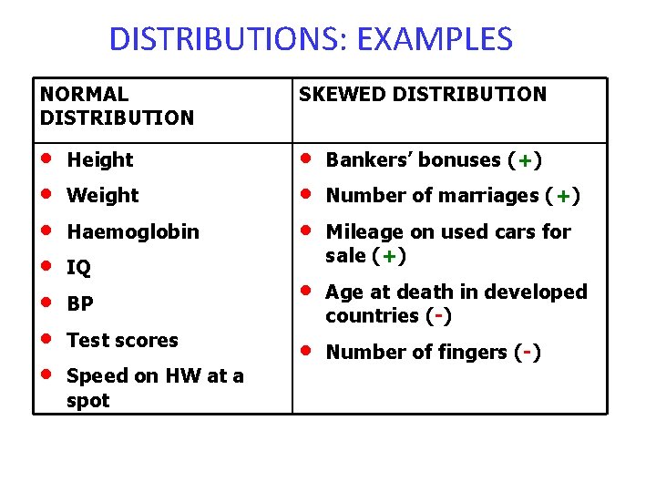
DISTRIBUTIONS: EXAMPLES NORMAL DISTRIBUTION SKEWED DISTRIBUTION • • • Bankers’ bonuses (+) • Age at death in developed countries (-) • Number of fingers (-) Height Weight Haemoglobin IQ BP Test scores Speed on HW at a spot Number of marriages (+) Mileage on used cars for sale (+)

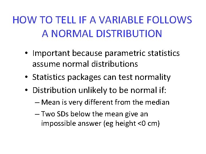
HOW TO TELL IF A VARIABLE FOLLOWS A NORMAL DISTRIBUTION • Important because parametric statistics assume normal distributions • Statistics packages can test normality • Distribution unlikely to be normal if: – Mean is very different from the median – Two SDs below the mean give an impossible answer (eg height <0 cm)

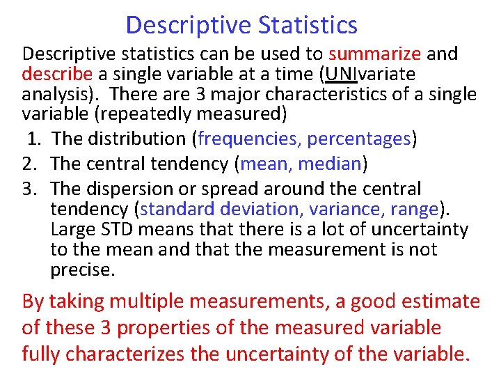
Descriptive Statistics Descriptive statistics can be used to summarize and describe a single variable at a time (UNIvariate analysis). There are 3 major characteristics of a single variable (repeatedly measured) 1. The distribution (frequencies, percentages) 2. The central tendency (mean, median) 3. The dispersion or spread around the central tendency (standard deviation, variance, range). Large STD means that there is a lot of uncertainty to the mean and that the measurement is not precise. By taking multiple measurements, a good estimate of these 3 properties of the measured variable fully characterizes the uncertainty of the variable.

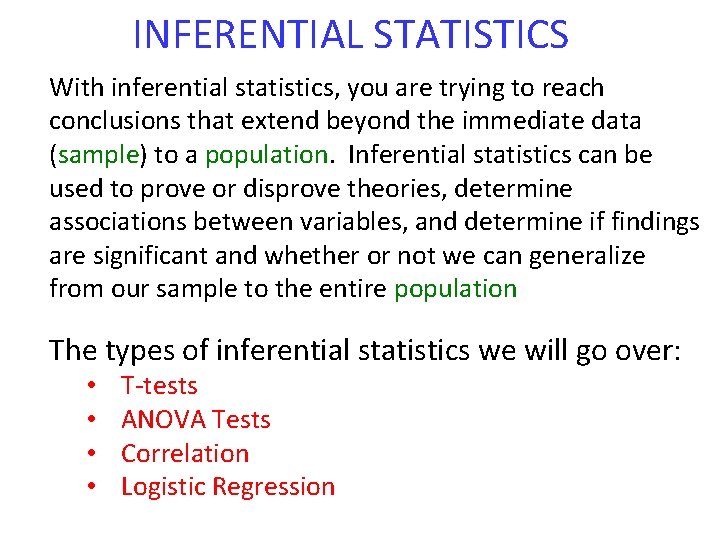
INFERENTIAL STATISTICS With inferential statistics, you are trying to reach conclusions that extend beyond the immediate data (sample) to a population. Inferential statistics can be used to prove or disprove theories, determine associations between variables, and determine if findings are significant and whether or not we can generalize from our sample to the entire population The types of inferential statistics we will go over: • • T-tests ANOVA Tests Correlation Logistic Regression

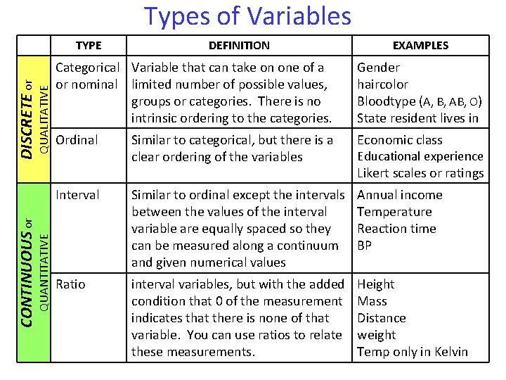
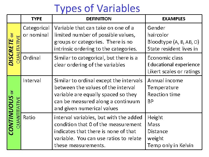
Types of Variables QUANTITATIVE CONTINUOUS or QUALITATIVE DISCRETE or TYPE DEFINITION EXAMPLES Categorical Variable that can take on one of a or nominal limited number of possible values, groups or categories. There is no intrinsic ordering to the categories. Gender haircolor Bloodtype (A, B, AB, O) State resident lives in Ordinal Similar to categorical, but there is a clear ordering of the variables Economic class Interval Similar to ordinal except the intervals between the values of the interval variable are equally spaced so they can be measured along a continuum and given numerical values Annual income Temperature Reaction time BP Ratio interval variables, but with the added condition that 0 of the measurement indicates that there is none of that variable. You can use ratios to relate these measurements. Height Mass Distance weight Temp only in Kelvin Educational experience Likert scales or ratings

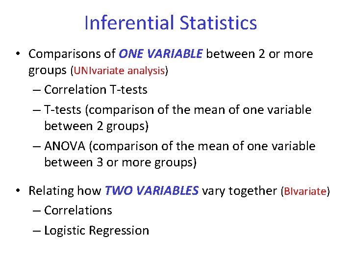
Inferential Statistics • Comparisons of ONE VARIABLE between 2 or more groups (UNIvariate analysis) – Correlation T-tests – T-tests (comparison of the mean of one variable between 2 groups) – ANOVA (comparison of the mean of one variable between 3 or more groups) • Relating how TWO VARIABLES vary together (BIvariate) – Correlations – Logistic Regression

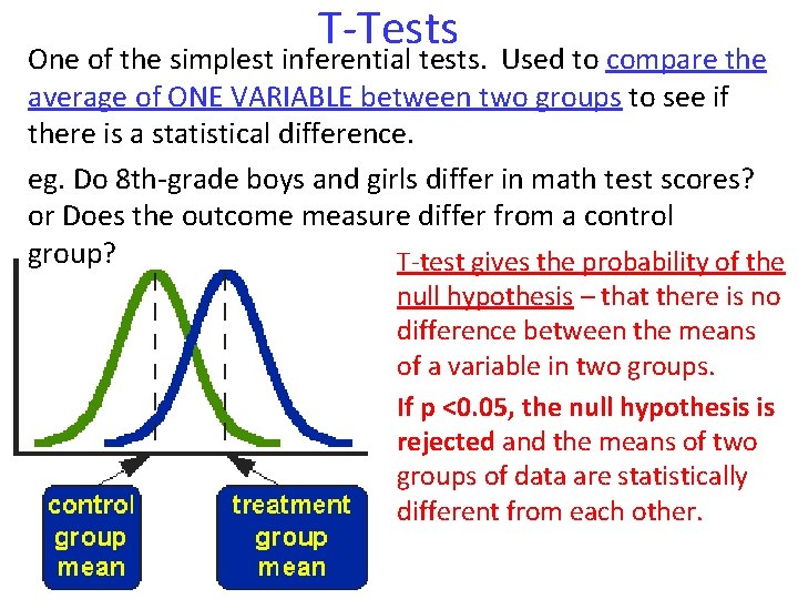
T-Tests One of the simplest inferential tests. Used to compare the average of ONE VARIABLE between two groups to see if there is a statistical difference. eg. Do 8 th-grade boys and girls differ in math test scores? or Does the outcome measure differ from a control group? T-test gives the probability of the null hypothesis – that there is no difference between the means of a variable in two groups. If p <0. 05, the null hypothesis is rejected and the means of two groups of data are statistically different from each other.

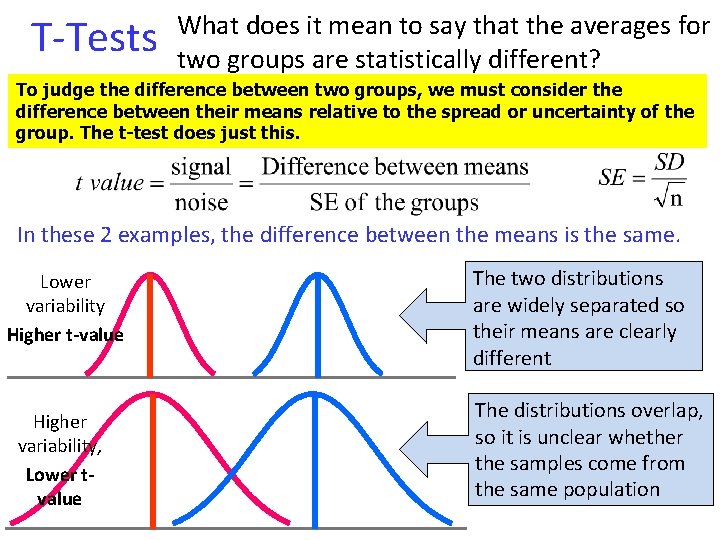
T-Tests What does it mean to say that the averages for two groups are statistically different? To judge the difference between two groups, we must consider the difference between their means relative to the spread or uncertainty of the group. The t-test does just this. In these 2 examples, the difference between the means is the same. Lower variability Higher t-value Higher variability, Lower tvalue The two distributions are widely separated so their means are clearly different The distributions overlap, so it is unclear whether the samples come from the same population

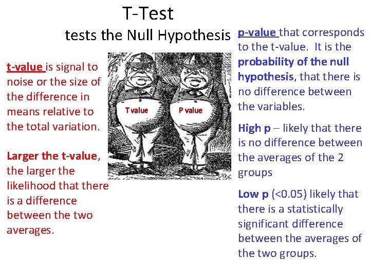
T-Test tests the Null Hypothesis t-value is signal to noise or the size of the difference in means relative to the total variation. Larger the t-value, the larger the likelihood that there is a difference between the two averages. p-value that corresponds to the t-value. It is the probability of the null hypothesis, that there is no difference between the variables. High p – likely that there is no difference between the averages of the 2 groups Low p (<0. 05) likely that there is a statistically significant difference between the averages of the two groups.

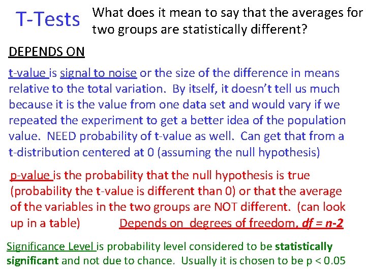
T-Tests What does it mean to say that the averages for two groups are statistically different? DEPENDS ON t-value is signal to noise or the size of the difference in means relative to the total variation. By itself, it doesn’t tell us much because it is the value from one data set and would vary if we repeated the experiment to get a better idea of the population value. NEED probability of t-value as well. Can get that from a t-distribution centered at 0 (assuming the null hypothesis) p-value is the probability that the null hypothesis is true (probability the t-value is different than 0) or that the average of the variables in the two groups are NOT different. (can look up in a table) Depends on degrees of freedom, df = n-2 Significance Level is probability level considered to be statistically significant and not due to chance. Usually it is chosen to be p < 0. 05

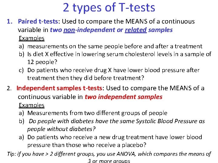
2 types of T-tests 1. Paired t-tests: Used to compare the MEANS of a continuous variable in two non-independent or related samples Examples a) measurements on the same people before and after a treatment b) Is diet X effective in lowering serum cholesterol levels in a sample of 12 people? c) Do patients who receive drug X have lower blood pressure after treatment then they did before treatment? 2. Independent samples t-tests: Used to compare the MEANS of a continuous variable in two independent samples Examples a) Measurements from two different groups of people b) Do people with diabetes have the same Systolic Blood Pressure as people without diabetes? a) Do patients who receive a new drug treatment have lower blood pressure than those who receive a placebo? Tip: if you have > 2 different groups, you use ANOVA, which compares the means of

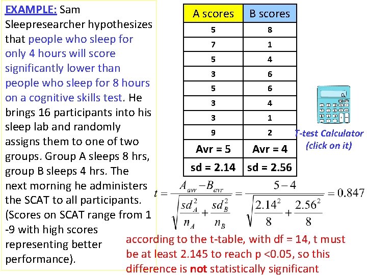
EXAMPLE: Sam A scores B scores Sleepresearcher hypothesizes 5 8 that people who sleep for 7 1 only 4 hours will score 5 4 significantly lower than 3 6 people who sleep for 8 hours 5 6 on a cognitive skills test. He 3 4 brings 16 participants into his 3 1 sleep lab and randomly 9 2 T-test Calculator assigns them to one of two Avr = 5 Avr = 4 (click on it) groups. Group A sleeps 8 hrs, sd = 2. 14 sd = 2. 56 group B sleeps 4 hrs. The next morning he administers the SCAT to all participants. (Scores on SCAT range from 1 -9 with high scores according to the t-table, with df = 14, t must representing better be at least 2. 145 to reach p <0. 05, so this performance). difference is not statistically significant

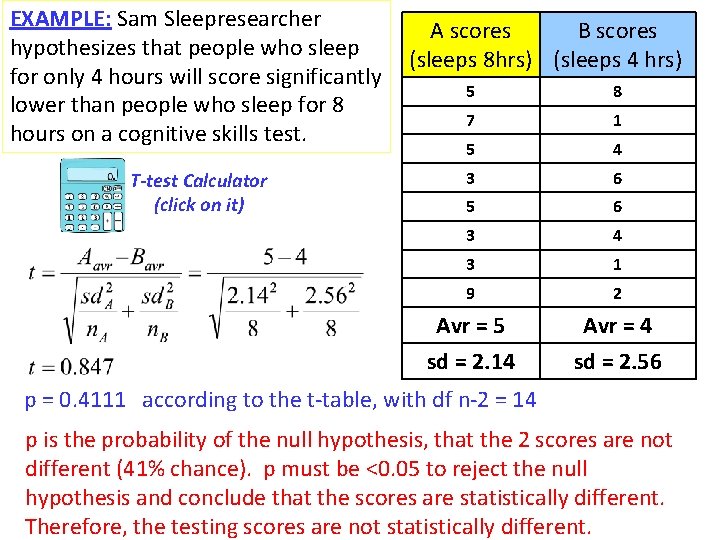
EXAMPLE: Sam Sleepresearcher A scores B scores hypothesizes that people who sleep (sleeps 8 hrs) (sleeps 4 hrs) for only 4 hours will score significantly 5 8 lower than people who sleep for 8 7 1 hours on a cognitive skills test. T-test Calculator (click on it) 5 4 3 6 5 6 3 4 3 1 9 2 Avr = 5 sd = 2. 14 Avr = 4 sd = 2. 56 p = 0. 4111 according to the t-table, with df n-2 = 14 p is the probability of the null hypothesis, that the 2 scores are not different (41% chance). p must be <0. 05 to reject the null hypothesis and conclude that the scores are statistically different. Therefore, the testing scores are not statistically different.

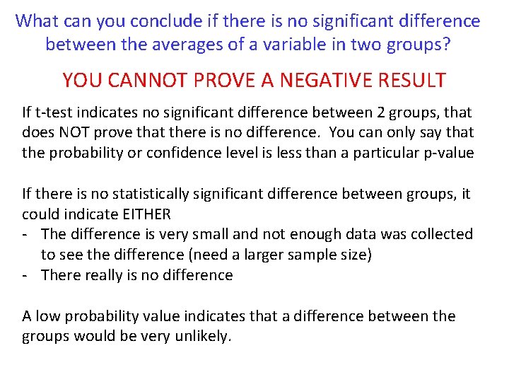
What can you conclude if there is no significant difference between the averages of a variable in two groups? YOU CANNOT PROVE A NEGATIVE RESULT If t-test indicates no significant difference between 2 groups, that does NOT prove that there is no difference. You can only say that the probability or confidence level is less than a particular p-value If there is no statistically significant difference between groups, it could indicate EITHER - The difference is very small and not enough data was collected to see the difference (need a larger sample size) - There really is no difference A low probability value indicates that a difference between the groups would be very unlikely.

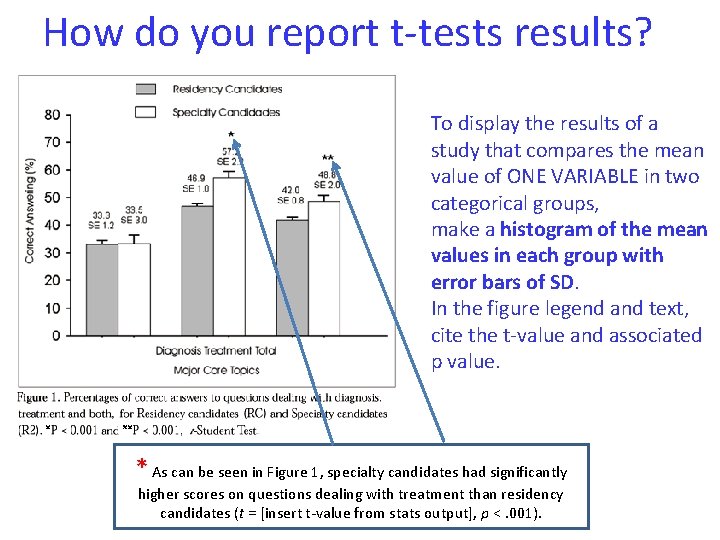
How do you report t-tests results? To display the results of a study that compares the mean value of ONE VARIABLE in two categorical groups, make a histogram of the mean values in each group with error bars of SD. In the figure legend and text, cite the t-value and associated p value. * As can be seen in Figure 1, specialty candidates had significantly higher scores on questions dealing with treatment than residency candidates (t = [insert t-value from stats output], p <. 001).

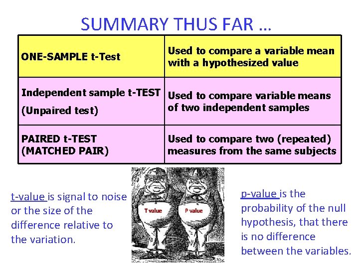
SUMMARY THUS FAR … ONE-SAMPLE t-Test Used to compare a variable mean with a hypothesized value Independent sample t-TEST Used to compare variable means of two independent samples (Unpaired test) PAIRED t-TEST (MATCHED PAIR) t-value is signal to noise or the size of the difference relative to the variation. Used to compare two (repeated) measures from the same subjects p-value is the probability of the null hypothesis, that there is no difference between the variables.

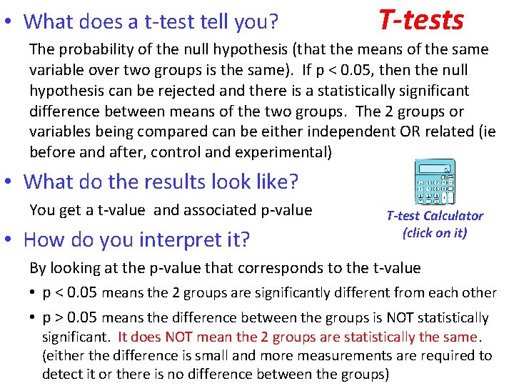
• What does a t-test tell you? T-tests The probability of the null hypothesis (that the means of the same variable over two groups is the same). If p < 0. 05, then the null hypothesis can be rejected and there is a statistically significant difference between means of the two groups. The 2 groups or variables being compared can be either independent OR related (ie before and after, control and experimental) • What do the results look like? You get a t-value and associated p-value • How do you interpret it? T-test Calculator (click on it) By looking at the p-value that corresponds to the t-value • p < 0. 05 means the 2 groups are significantly different from each other • p > 0. 05 means the difference between the groups is NOT statistically significant. It does NOT mean the 2 groups are statistically the same. (either the difference is small and more measurements are required to detect it or there is no difference between the groups)

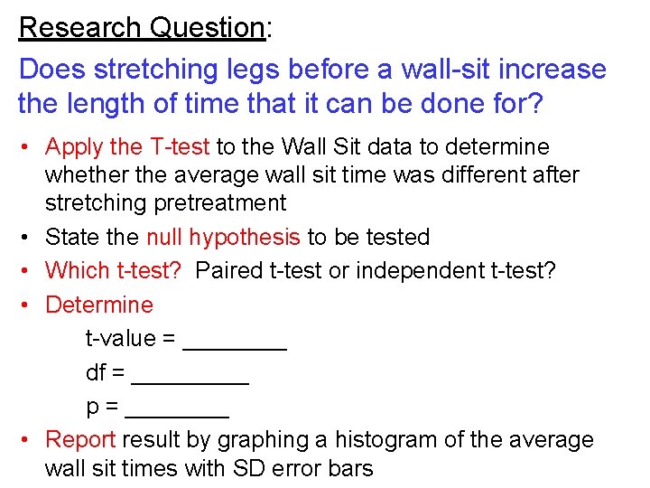
Research Question: Does stretching legs before a wall-sit increase the length of time that it can be done for? • Apply the T-test to the Wall Sit data to determine whether the average wall sit time was different after stretching pretreatment • State the null hypothesis to be tested • Which t-test? Paired t-test or independent t-test? • Determine t-value = ____ df = _____ p = ____ • Report result by graphing a histogram of the average wall sit times with SD error bars

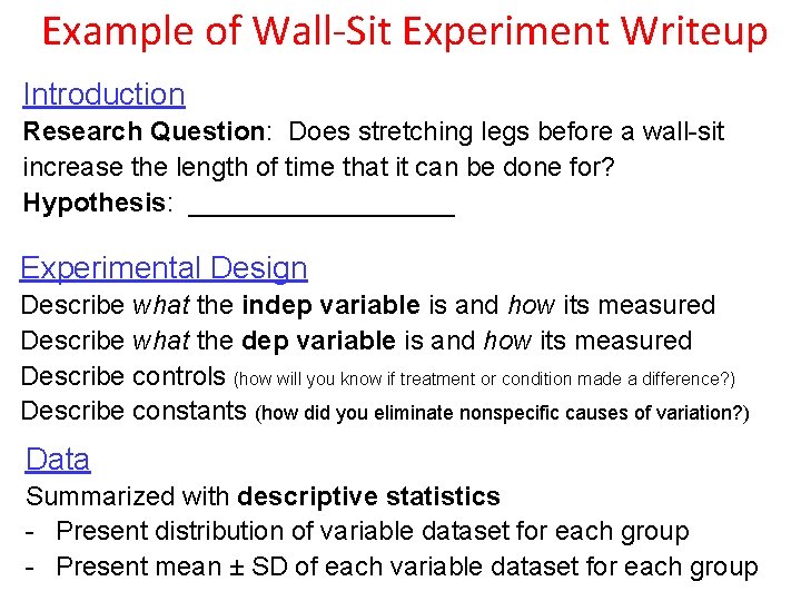
Example of Wall-Sit Experiment Writeup Introduction Research Question: Does stretching legs before a wall-sit increase the length of time that it can be done for? Hypothesis: _________ Experimental Design Describe what the indep variable is and how its measured Describe what the dep variable is and how its measured Describe controls (how will you know if treatment or condition made a difference? ) Describe constants (how did you eliminate nonspecific causes of variation? ) Data Summarized with descriptive statistics - Present distribution of variable dataset for each group - Present mean ± SD of each variable dataset for each group

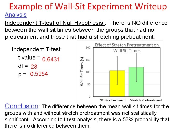
Example of Wall-Sit Experiment Writeup Analysis Independent T-test of Null Hypothesis : There is NO difference between the wall sit times between the groups that had no pretreatment and those that had a stretching pretreatment. Independent T-test t-value = 0. 6431 df = 28 p = 0. 5254 Conclusion: The difference between the mean wall sit times for the groups with and without stretch pretreatment was not statistically significant. According to t-test analysis, there is a 53% probability that there is no difference between them.

Alphabet Practice Experiment • For this experiment, we use one group, who will perform an experiment six times. • You will be issued with a piece of paper with the task on it. Do not turn it over until instructed. • You will need a pen to write on your recording sheet. • Each attempt needs to be timed, and the time recorded.

Alphabet Practice Experiment Time how long it takes to find the letters A to Z in order.

Alphabet Practice Experiment Recording times to find the letters of the alphabet in order 1. What do you think the research question is? 2. What is the treatment (independent variable)? What is the response variable (dependent variable)? 3. What do you think the outcome will be? (Hypothesis)

Alphabet Practice Experiment DATA - Record and display class data in table - Show Descriptive Statistics of the dependent variable for 2 groups a) show the distribution (with box and whiskers plots or frequency histograms) b) Determine the mean value of each dataset c) Quantify the average dispersion of each variable dataset with SD

Alphabet Practice Experiment ANALYSIS • Apply the T-test to the Alphabet Practice Experiment • State the null hypothesis to be tested • Which t-test? Paired t-test or independent t-test? • Determine t-value = ____ df = _____ p = ____ • Report result by graphing a histogram of the average values with SD error bars • State your conclusions to the experiment and support with evidence.

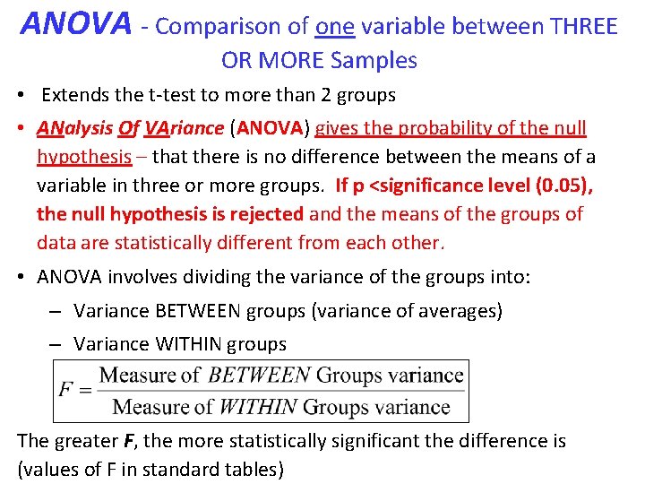
ANOVA - Comparison of one variable between THREE OR MORE Samples • Extends the t-test to more than 2 groups • ANalysis Of VAriance (ANOVA) gives the probability of the null hypothesis – that there is no difference between the means of a variable in three or more groups. If p <significance level (0. 05), the null hypothesis is rejected and the means of the groups of data are statistically different from each other. • ANOVA involves dividing the variance of the groups into: – Variance BETWEEN groups (variance of averages) – Variance WITHIN groups The greater F, the more statistically significant the difference is (values of F in standard tables)

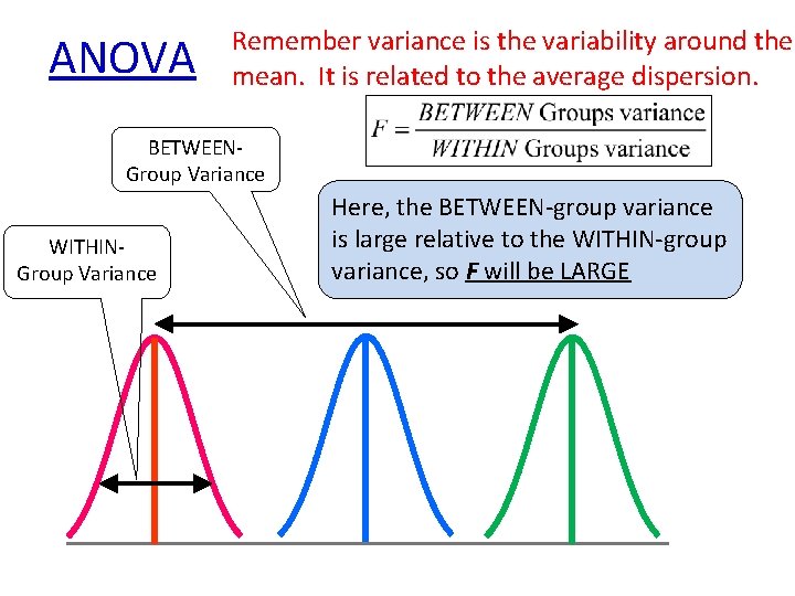
ANOVA Remember variance is the variability around the mean. It is related to the average dispersion. BETWEENGroup Variance WITHINGroup Variance Here, the BETWEEN-group variance is large relative to the WITHIN-group variance, so F will be LARGE

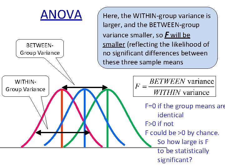
ANOVA BETWEENGroup Variance Here, the WITHIN-group variance is larger, and the BETWEEN-group variance smaller, so F will be smaller (reflecting the likelihood of no significant differences between these three sample means WITHINGroup Variance F=0 if the group means are identical F>0 if not F could be >0 by chance. So how large is F to be statistically significant?

ANOVA DEPENDS ON What does it mean to say that the averages for three or more groups are statistically different? F-value ratio of between group variance to within group variance. By itself it doesn’t tell us much because it is the value from one data set and would vary if we repeated the experiment to get a better idea of the population value. NEED probability of F value as well. Can get that from a distribution of F-values centered at 0 (assuming the null hypothesis) p-value is the probability that the null hypothesis is true (probability the F-value is different than 0) or that the means of the variable in the multiple groups are NOT different. (can look up in a table) Depends on degrees of freedom, df: (dfbetw=ngroup-1; dfwithin = ntotal-1 -dfbetw) Significance Level is probability level considered to be statistically significant and not due to chance. Usually it is chosen to be p < 0. 05

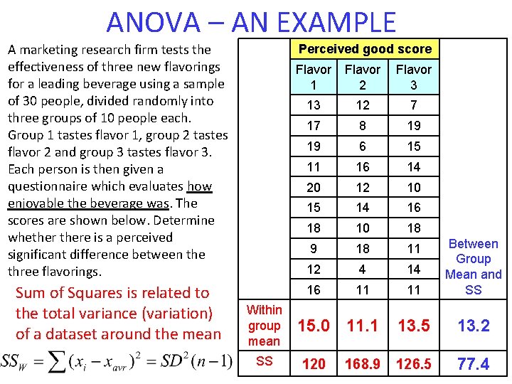
ANOVA – AN EXAMPLE A marketing research firm tests the effectiveness of three new flavorings for a leading beverage using a sample of 30 people, divided randomly into three groups of 10 people each. Group 1 tastes flavor 1, group 2 tastes flavor 2 and group 3 tastes flavor 3. Each person is then given a questionnaire which evaluates how enjoyable the beverage was. The scores are shown below. Determine whethere is a perceived significant difference between the three flavorings. Sum of Squares is related to the total variance (variation) of a dataset around the mean Perceived good score Within group mean SS Flavor 1 Flavor 2 Flavor 3 13 12 7 17 8 19 19 6 15 11 16 14 20 12 10 15 14 16 18 10 18 9 18 11 12 4 14 16 11 11 Between Group Mean and SS 13. 5 13. 2 126. 5 77. 4 15. 0 11. 1 120 168. 9

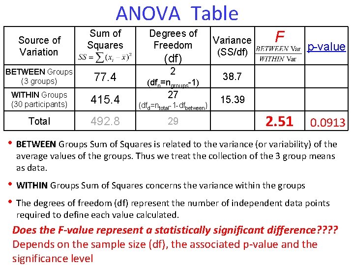
ANOVA Table Source of Variation Sum of Squares Degrees of Freedom (df) BETWEEN Groups (3 groups) 77. 4 WITHIN Groups (30 participants) 415. 4 Total 492. 8 2 (dfn=ngroups-1) 27 (dfd=ntotal-1 -dfbetween) 29 Variance (SS/df) F p-value 38. 7 15. 39 2. 51 0. 0913 • BETWEEN Groups Sum of Squares is related to the variance (or variability) of the average values of the groups. Thus we treat the collection of the 3 group means as data. • WITHIN Groups Sum of Squares concerns the variance within the groups • The degrees of freedom (df) represent the number of independent data points required to define each value calculated. Does the F-value represent a statistically significant difference? ? Depends on the sample size (df), the associated p-value and the significance level

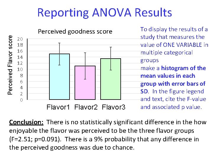
Perceived Flavor score Reporting ANOVA Results 20 18 16 14 12 10 8 6 4 2 0 Perceived goodness score Flavor 1 Flavor 2 Flavor 3 To display the results of a study that measures the value of ONE VARIABLE in multiple categorical groups make a histogram of the mean values in each group with error bars of SD. In the figure legend and text, cite the F-value and associated p value. Conclusion: There is no statistically significant difference in the how enjoyable the flavor was perceived to be three flavor groups (F=2. 51; p=0. 091). There is a 9% probability that any difference in the perceived goodness was due to chance.

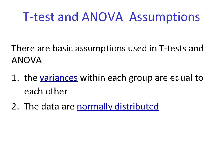
T-test and ANOVA Assumptions There are basic assumptions used in T-tests and ANOVA 1. the variances within each group are equal to each other 2. The data are normally distributed

Inferential Statistics Correlation and Regression (BIVARIATE Analysis) T-tests and ANOVA compare one variable between 2 or more groups eg. Comparison of BP in females and males or Comparison of BP before and after a drug Correlation and regression analyses are used to see how two variables vary together. Eg. How are the variables BP and Heart Rate related

Correlation One of the most common and most useful statistics. A correlation is a single number that describes the degree of relationship between two variables. It is NOT related to cause and effect. • When to use it? When you want to know about the association or relationship between two continuous variables egs. Relationship between food intake and weight; drug dosage and blood pressure air temp and metabolic rate • What does it tell you? If a linear relationship exists between two variables, and how strong that relationship is. • What do the results look like? – The correlation coefficient = Pearson’s r can use CORREL() function in Excel to find r – Pearson’s coefficient, r, ranges from -1 to +1

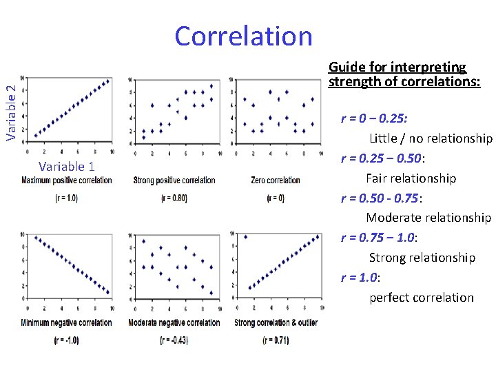
Correlation Variable 2 Guide for interpreting strength of correlations: Variable 1 r = 0 – 0. 25: Little / no relationship r = 0. 25 – 0. 50: Fair relationship r = 0. 50 - 0. 75: Moderate relationship r = 0. 75 – 1. 0: Strong relationship r = 1. 0: perfect correlation

Correlation • How do you interpret it? a) If r is positive, high values of one variable are associated with high values of the other variable (both go in SAME direction: ↑↑ OR ↓↓) Eg. Diastolic blood pressure tends to rise with age, thus the two variables are positively correlated b) If r is negative, low values of one variable are associated with high values of the other variable (variables change in opposite direction: ↑↓ OR ↓ ↑) Eg. Heart rate tends to be lower in persons who exercise frequently, the two variables correlate negatively c) r=0: Correlation of 0 indicates NO linear relationship • How do you report it? “Diastolic blood pressure was positively correlated with age (r =. 75, p <. 05). ” Tip: Correlation does NOT equal causation!!! If two variables are highly correlated, this does NOT mean that one CAUSES the other!!! NO Correlation does NOT mean no relationship

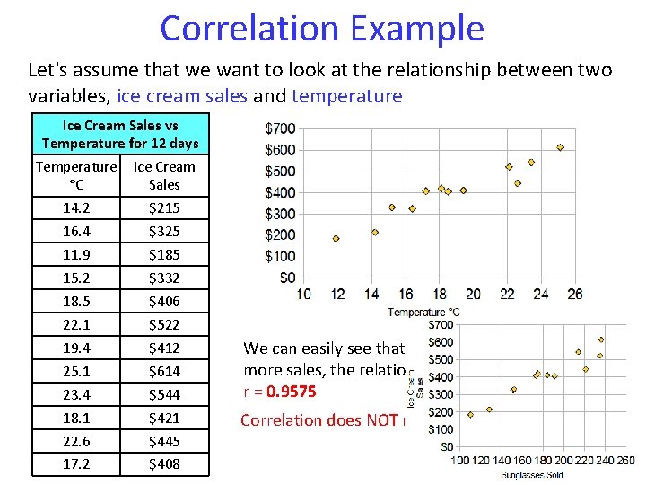
Correlation Example Let's assume that we want to look at the relationship between two variables, ice cream sales and temperature Ice Cream Sales vs Temperature for 12 days Temperature Ice Cream °C Sales 14. 2 $215 16. 4 $325 11. 9 $185 15. 2 $332 18. 5 $406 22. 1 $522 19. 4 $412 25. 1 $614 23. 4 $544 We can easily see that warmer weather leads to more sales, the relationship is good but not perfect. r = 0. 9575 18. 1 $421 Correlation does NOT mean causation 22. 6 $445 17. 2 $408

Correlation Significance How statistically significant is the correlation value? Depends on - significance level (usually 0. 05 which is the probability that the correlation occurred by chance. p<5% is defined as statistically significant and not due to chance) - df or sample size (degrees of freedom) you can look in a table of r values to see if the r is large enough to say that the difference between the groups is significant and not likely to have been due to chance (p<0. 05)

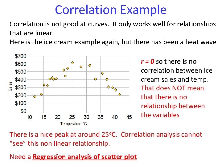
Correlation Example Correlation is not good at curves. It only works well for relationships that are linear. Here is the ice cream example again, but there has been a heat wave r = 0 so there is no correlation between ice cream sales and temp. That does NOT mean that there is no relationship between the variables There is a nice peak at around 25 o. C. Correlation analysis cannot “see” this non linear relationship. Need a Regression analysis of scatter plot

Regression analysis is a statistical process for estimating the relationships among variables. It includes many techniques for modeling and analyzing several variables, when the focus is on the relationship between a dependent variable and one or more independent variables. • When to use it? When you want to mathematically model the relationship between any continuous independent and dependent variable • What does it tell you? The mathematical relationship between two continuous variables. • What do the results look like? – The two variables are graphed on a scatter plot – The data is fit with a curve of best fit – The mathematical function that describes the curve of best fit is a mathematical model of the relationship between the indep and dep variable and the R 2 value gives goodness of fit

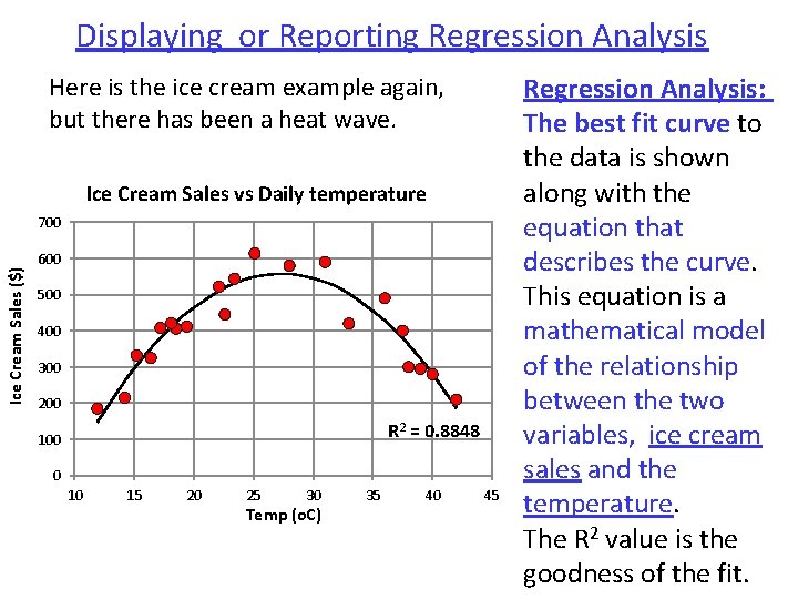
Displaying or Reporting Regression Analysis Here is the ice cream example again, but there has been a heat wave. Ice Cream Sales vs Daily temperature Ice Cream Sales ($) 700 600 500 400 300 200 R 2 = 0. 8848 100 0 10 15 20 25 30 Temp (o. C) 35 40 45 Regression Analysis: The best fit curve to the data is shown along with the equation that describes the curve. This equation is a mathematical model of the relationship between the two variables, ice cream sales and the temperature. The R 2 value is the goodness of the fit.