Basic Results in Probability and Statistics Summation and

Basic Results in Probability and Statistics

Summation and Product Operators

Probability
")
Random Variables (Univariate)

Bernoulli Distribution • An experiment consists of one trial. It can result in one of 2 outcomes: Success or Failure (or a characteristic being Present or Absent). • Probability of Success is p (0 < p < 1) • Y = 1 if Success (Characteristic Present), 0 if not
 qbinom(q, n, pi) dbinom(y, n, pi) rbinom(m,")
Binomial Distribution R Functions: pbinom(y, n, pi) qbinom(q, n, pi) dbinom(y, n, pi) rbinom(m, n, pi) P(Y ≤ y) qth quantile p(y) pseudo random sample of size m

Binomial Experiment • Experiment consists of a series of n identical Bernoulli trials • Each trial can end in one of 2 outcomes: Success or Failure • Trials are independent (outcome of one has no bearing on outcomes of others) • Probability of Success, p, is constant for all trials • Random Variable Y, is the number of Successes in the n trials is said to follow Binomial Distribution with parameters n and p • Y can take on the values y=0, 1, …, n Notation: Y~Bin(n, p)

Poisson Distribution • Distribution often used to model the number of incidences of some characteristic in time or space: • Arrivals of customers in a queue • Numbers of flaws in a roll of fabric • Number of typos per page of text. • Distribution obtained as follows: • • • Break down the “area” into many small “pieces” (n pieces) Each “piece” can have only 0 or 1 occurrences (p=P(1)) Let l=np ≡ Average number of occurrences over “area” Y ≡ # occurrences in “area” is sum of 0 s & 1 s over “pieces” Y ~ Bin(n, p) with p = l/n Take limit of Binomial Distribution as n with p = l/n

Negative Binomial Distribution • Used to model the number of Bernoulli trials needed until the rth Success occurs • Based on there being r-1 Successes in first y-1 trials, followed by a Success
 This model is widely used to model count data when")
Negative Binomial Distribution (II) This model is widely used to model count data when the Poisson model does not fit well due to over-dispersion: V(Y) > E(Y). In this model, k is not assumed to be integer-valued and must be estimated along with m
 Distribution • Bell-shaped distribution with tendency for individuals to clump around the")
Normal (Gaussian) Distribution • Bell-shaped distribution with tendency for individuals to clump around the group median/mean • Used to model many scientific phenomena • Many estimators have approximate normal sampling distributions (see Central Limit Theorem) • Notation: Y~N(m, s 2) where m is mean and s 2 is variance R Functions: pnorm(y, mu, sigma) qnorm(q, mu, sigma) dnorm(y, mu, sigma) rnorm(n, mu, sigma) P(Y ≤ y) qth quantile f(y) pseudo random sample of size n
")
Normal Distribution – Density Functions (pdf)

Second Decimal Place of z Integer part and first decimal place of z

Gamma Distribution • Family of Right-Skewed Distributions • Random Variable can take on positive values only • Used to model many biological and economic characteristics • Can take on many different shapes to match empirical data
: pgamma(y, alpha, beta) qgamma(q,")
Gamma Distribution – Mean and Variance R Functions (Model 2): pgamma(y, alpha, beta) qgamma(q, alpha, beta) dgamma(y, alpha, beta) rgamma(n, alpha, beta) P(Y ≤ y) qth quantile f(y) pseudo random sample of size n
")
Gamma/Exponential Densities (pdf)

Beta Distribution • Used to model proportions (can be generalized to any finite, positive range) • Parameters allow a wide range of shapes to model empirical data
")
Beta Density Functions (pdf)
 - I")
Random Variables (Bivariate) - I
 - II")
Random Variables (Bivariate) - II

Covariance, Correlation, Independence

Linear Functions of RVs - I

Linear Functions of RVs - II

Linear Functions of RVs - III

Functions of Normal Random Variables - I • Assume a random sample of size n from a Normal distribution with mean m and variance s 2 (random sample implies the observations are independent) • The sample mean and the sample variance are obtained. The following results hold (Casella & Berger (2002), Section 5. 3).
” X~cn 2 • Z~N(0, 1)")
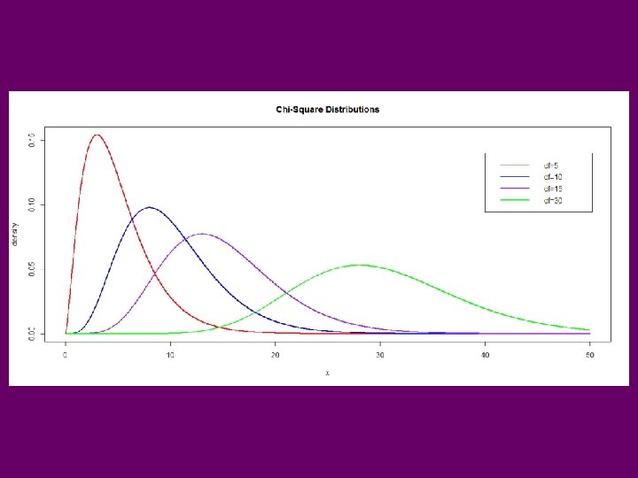
Chi-Square Distribution • Indexed by “degrees of freedom (n)” X~cn 2 • Z~N(0, 1) Z 2 ~c 12 • Assuming Independence: R Functions: pchisq(x, nu) qchisq(q, nu) dchisq(x, nu) rchisq(n, nu) P(X ≤ x) qth quantile f(x) pseudo random sample of size n
")
Critical Values for Chi-Square Distributions (Mean=n, Variance=2 n)
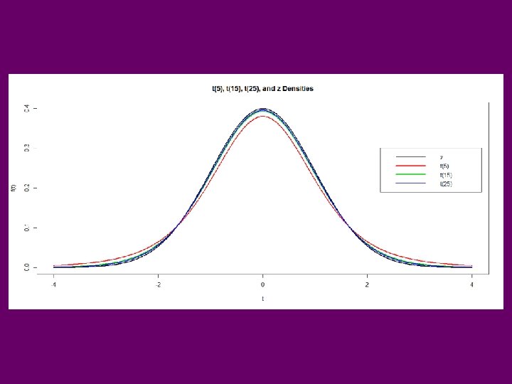
” X~tn • Z~N(0, 1), X~cn")
Student’s t-Distribution • Indexed by “degrees of freedom (n)” X~tn • Z~N(0, 1), X~cn 2 • Assuming Independence of Z and X: R Functions: pt(t, nu) qt(q, nu) dt(t, nu) rt(n, nu) P(T ≤ t) qth quantile f(t) pseudo random sample of size n

Critical Values for Student’s t-Distributions
 • Consider two (independent) random samples from two normal distributions with")
Comparing Variances (Ratios) • Consider two (independent) random samples from two normal distributions with the goal of comparing the population variances.
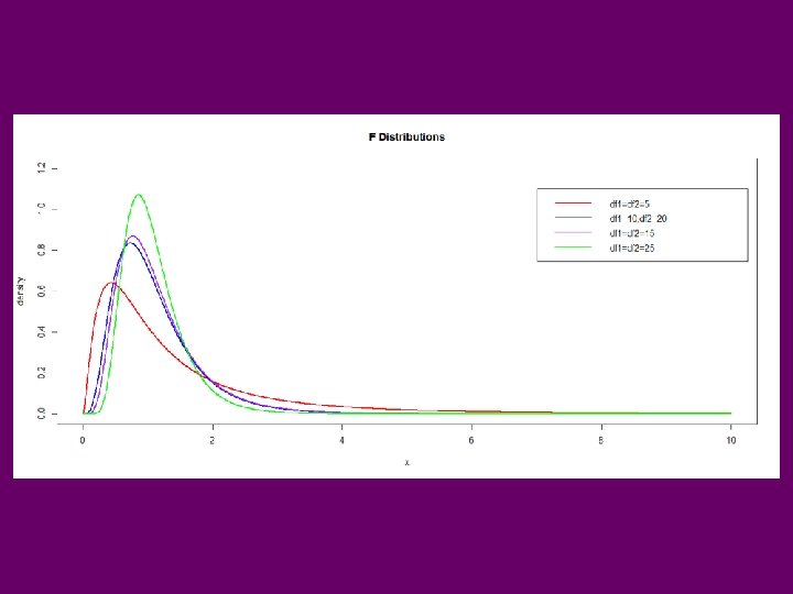
” W~Fn 1,")
F-Distribution • Indexed by 2 “degrees of freedom (n 1, n 2)” W~Fn 1, n 2 • X 1 ~cn 12, X 2 ~cn 22 • Assuming Independence of X 1 and X 2: R Functions: pf(w, nu 1, nu 2) qf(q, nu 1, nu 2) df(w, nu 1, nu 2) rf(n, nu 1, nu 2) P(W ≤ w) qth quantile f(w) pseudo random sample of size n
 = 0. 95")
Critical Values for F-distributions P(F ≤ Table Value) = 0. 95
 and")
Statistical Estimation - Properties Note: If an estimator is unbiased (easy to show) and its variance goes to zero as its sample size gets infinitely large (easy to show), it is consistent. It is tougher to show that it is Minimum Variance, but general results have been obtained in many standard cases.

Maximum Likelihood and Least Squares

One-Sample Confidence Interval for m • • SRS from Normal Distribution Y 1, …, Yn ~ NID(m, s 2) Sample mean, sample standard deviation are obtained Degrees of freedom are df= n-1 Level (1 -a) confidence interval of form: Procedure is theoretically derived based on normally distributed data, but has been found to work well regardless for moderate to large n
 • 2 -sided Test: H 0: m =")
1 -Sample t-test (2 -tailed alternative) • 2 -sided Test: H 0: m = m 0 • Decision Rule : H a: m m 0 § Conclude m > m 0 if Test Statistic (t*) > ta/2, n-1 § Conclude m < m 0 if Test Statistic (t*) <- -ta/2, n-1 § Do not conclude m m 0 otherwise • P-value: 2 P(tn-1 |tobs|) • Test Statistic:

Comparing 2 Means - Independent Samples - I

Comparing 2 Means - Independent Samples - II

Inference for m 1 -m 2 - Normal Populations – Equal variances • Interpretation (at the a significance level): § § § If interval contains 0, do not reject H 0: m 1 = m 2 If interval is strictly positive, conclude that m 1 > m 2 If interval is strictly negative, conclude that m 1 < m 2
")
Inference for s 2 (Normal Data)

Inferences Regarding 2 Population Variances

Central Limit Theorem • When random samples of size n are selected from any population with mean m and finite variance s 2, the sampling distribution of the sample mean will be approximately normally distributed for large n:
- Slides: 45