Basic regression modelling to evaluate programme impact Hctor

Basic regression modelling to evaluate programme impact Héctor Lamadrid Center for Population Health Research National Institute of Public Health, Mexico

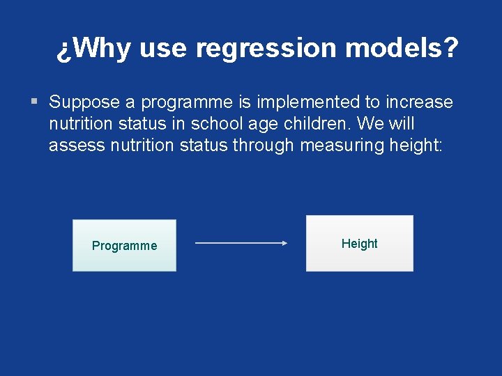
¿Why use regression models? § Suppose a programme is implemented to increase nutrition status in school age children. We will assess nutrition status through measuring height: Programme Height

How do we answer the question…? Did the programme have an impact on children’s height?

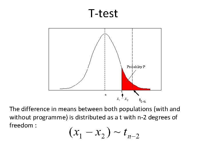
T-test 0 t 1 -a The difference in means between both populations (with and without programme) is distributed as a t with n-2 degrees of freedom :

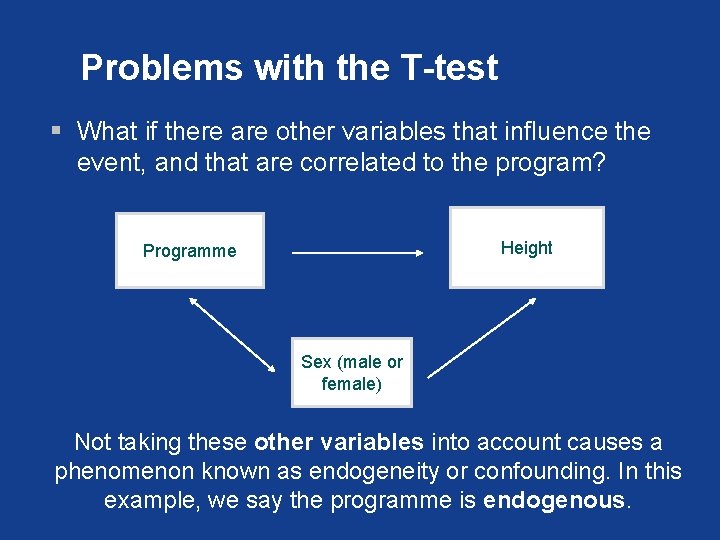
Problems with the T-test § What if there are other variables that influence the event, and that are correlated to the program? Height Programme Sex (male or female) Not taking these other variables into account causes a phenomenon known as endogeneity or confounding. In this example, we say the programme is endogenous.

Endogeneity Example: § We know girls of school age tend to be taller than boys. § For some reason there are more girls than boys enrolled in the programme. § When we compare those who have a programme to those who do not have it, those enrolled have a greater height in average. § Is this difference attributable to the programme? How can we be sure?

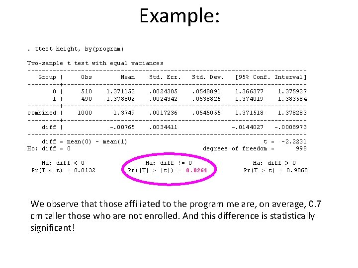
Example: . ttest height, by(program) Two-sample t test with equal variances ---------------------------------------Group | Obs Mean Std. Err. Std. Dev. [95% Conf. Interval] -----+----------------------------------0 | 510 1. 371152. 0024305. 0548891 1. 366377 1. 375927 1 | 490 1. 378802. 0024342. 0538826 1. 374019 1. 383584 -----+----------------------------------combined | 1000 1. 3749. 0017236. 0545055 1. 371518 1. 378283 -----+----------------------------------diff | -. 00765. 0034411 -. 0144027 -. 0008973 ---------------------------------------diff = mean(0) - mean(1) t = -2. 2231 Ho: diff = 0 degrees of freedom = 998 Ha: diff < 0 Pr(T < t) = 0. 0132 Ha: diff != 0 Pr(|T| > |t|) = 0. 0264 Ha: diff > 0 Pr(T > t) = 0. 9868 We observe that those affiliated to the program me are, on average, 0. 7 cm taller those who are not enrolled. And this difference is statistically significant!

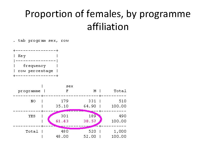
Proportion of females, by programme affiliation. tab program sex, row +--------+ | Key | |--------| | frequency | | row percentage | +--------+ | sex programme | F M | Total ------+-----------+-----NO | 179 331 | 510 | 35. 10 64. 90 | 100. 00 ------+-----------+-----YES | 301 189 | 490 | 61. 43 38. 57 | 100. 00 ------+-----------+-----Total | 480 520 | 1, 000 | 48. 00 52. 00 | 100. 00

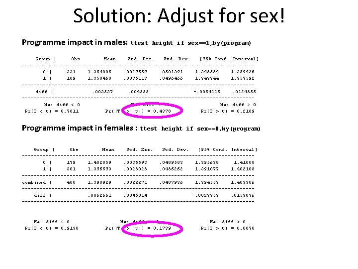
Solution: Adjust for sex! Programme impact in males: ttest height if sex==1, by(program) Group | Obs Mean Std. Err. Std. Dev. [95% Conf. Interval] -----+----------------------------------0 | 331 1. 354005. 0027559. 0501391 1. 348584 1. 359426 1 | 189 1. 350468. 0036113. 0496466 1. 343344 1. 357592 -----+----------------------------------diff |. 003537. 004555 -. 0054115. 0124855 ---------------------------------------Ha: diff < 0 Ha: diff != 0 Ha: diff > 0 Pr(T < t) = 0. 7811 Pr(|T| > |t|) = 0. 4378 Pr(T > t) = 0. 2189 Programme impact in females : ttest height if sex==0, by(program) Group | Obs Mean Std. Err. Std. Dev. [95% Conf. Interval] -----+----------------------------------0 | 179 1. 402859. 0036593. 0489583 1. 395638 1. 41008 1 | 301 1. 396593. 0028028. 0486262 1. 391077 1. 402108 -----+----------------------------------combined | 480 1. 398929. 0022271. 0487936 1. 394553 1. 403306 -----+----------------------------------diff |. 0062661. 0046014 -. 0027753. 0153076 --------------------------------------- Ha: diff < 0 Pr(T < t) = 0. 9130 Ha: diff != 0 Pr(|T| > |t|) = 0. 1739 Ha: diff > 0 Pr(T > t) = 0. 0870

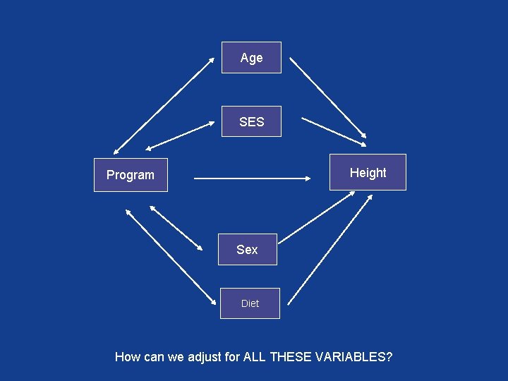
Age SES Height Program Sex Diet How can we adjust for ALL THESE VARIABLES?

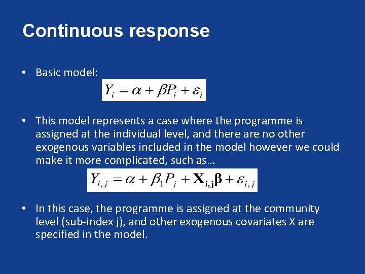
Continuous response • Basic model: • This model represents a case where the programme is assigned at the individual level, and there are no other exogenous variables included in the model however we could make it more complicated, such as… • In this case, the programme is assigned at the community level (sub-index j), and other exogenous covariates X are specified in the model.

Continuous response § In both cases, such a model could be estimated by linear regression § The method of estimation used is known as Ordinary Least Squares § In the econometric literature (as opposed to biostatistical or epidemiological) the term OLS regression is more common than linear regression, although both terms represent the same thing.

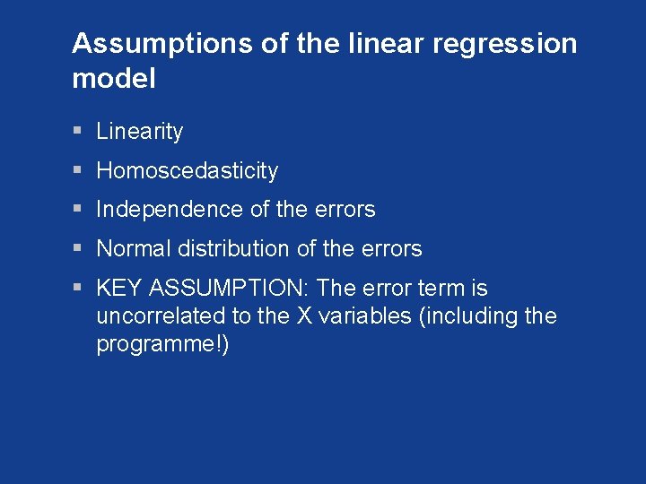
Assumptions of the linear regression model § Linearity § Homoscedasticity § Independence of the errors § Normal distribution of the errors § KEY ASSUMPTION: The error term is uncorrelated to the X variables (including the programme!)

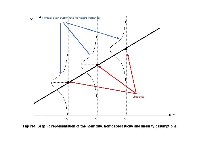
Y Normal distribution and constant variance Linearity X x 1 x 2 x 3 Figure 1. Graphic representation of the normality, homoscedasticity and linearity assumptions.

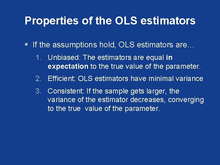
Properties of the OLS estimators § If the assumptions hold, OLS estimators are… 1. Unbiased: The estimators are equal in expectation to the true value of the parameter. 2. Efficient: OLS estimators have minimal variance 3. Consistent: If the sample gets larger, the variance of the estimator decreases, converging to the true value of the parameter.

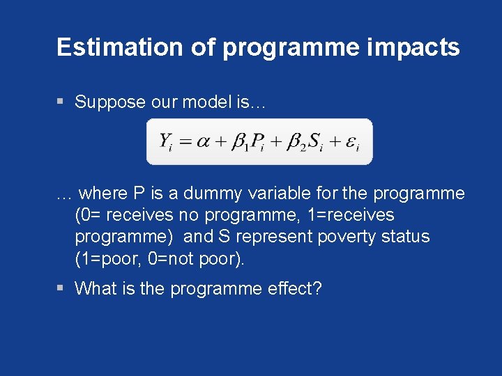
Estimation of programme impacts § Suppose our model is… … where P is a dummy variable for the programme (0= receives no programme, 1=receives programme) and S represent poverty status (1=poor, 0=not poor). § What is the programme effect?

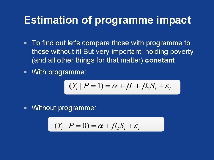
Estimation of programme impact § To find out let’s compare those with programme to those without it! But very important: holding poverty (and all other things for that matter) constant § With programme: § Without programme:

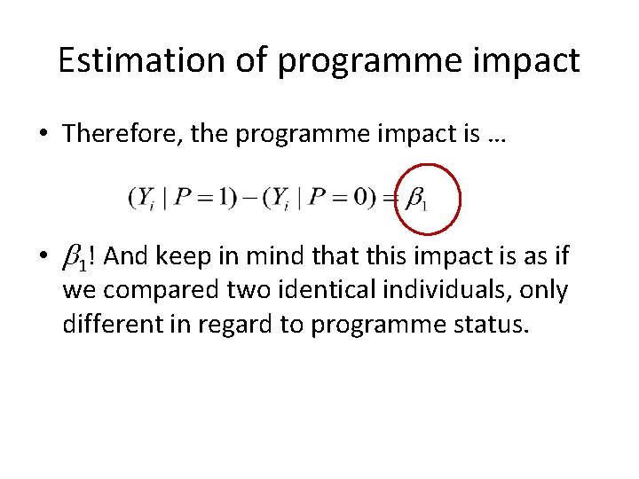
Estimation of programme impact • Therefore, the programme impact is … • b 1! And keep in mind that this impact is as if we compared two identical individuals, only different in regard to programme status.

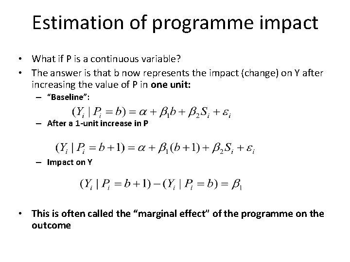
Estimation of programme impact • What if P is a continuous variable? • The answer is that b now represents the impact (change) on Y after increasing the value of P in one unit: – “Baseline”: – After a 1 -unit increase in P – Impact on Y • This is often called the “marginal effect” of the programme on the outcome

Including explanatory dummy variables in the model § Some variable are naturally dichotomous or categorical § However, sometimes it is desirable to categorize continuous variables to accomodate for nonlinear effects § Allows for heterogeneous impact estimations (will expand on this a little later)

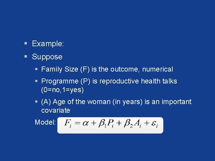
§ Example: § Suppose § Family Size (F) is the outcome, numerical § Programme (P) is reproductive health talks (0=no, 1=yes) § (A) Age of the woman (in years) is an important covariate Model:

§ The problem with this especification is that due to the linearity assumption, the effect of a 1 year increase in age is supposed to be the same regardless of the age range! § This contradicts what has been observed because it implies that family size increases ad infinitum!, lets look at the truth…

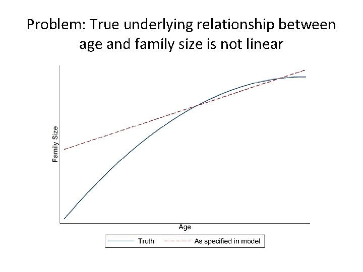
Problem: True underlying relationship between age and family size is not linear

§ The solution is to generate a categorical variable with the following values, for example: § 1 if age is between 15 and 24 § 2 if age is between 25 and 35 § 3 if age is between 36 and 49 § CAUTION: Do not include the categorical value itself in the model! (it would force us to make a new, unrealistic, linearity assumption)

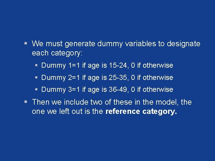
§ We must generate dummy variables to designate each category: § Dummy 1=1 if age is 15 -24, 0 if otherwise § Dummy 2=1 if age is 25 -35, 0 if otherwise § Dummy 3=1 if age is 36 -49, 0 if otherwise § Then we include two of these in the model, the one we left out is the reference category.

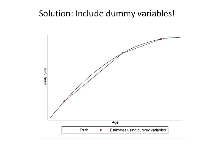
Solution: Include dummy variables!

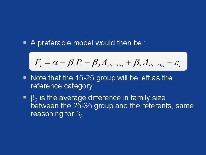
§ A preferable model would then be : § Note that the 15 -25 group will be left as the reference category § b 2 is the average difference in family size between the 25 -35 group and the referents, same reasoning for b 3

Heterogeneous impact § The programme may have a different impact in particular subgroups of the population § What if its impact is different in urban and rural areas? § We need to evelaute the possibility of this heterogeneous impact (a. k. a interaction, a. k. a. effect modification), so we must re-specify our model to accomodate for this…

Heterogeneous impact § We want to know if the effect of the programme is different in rural areas than in urban areas. § We need to include an interaction variable in the model, that is: the product of the programme dummy and the rural/urban dummy variable (Ri {1=rural, 0=urban})

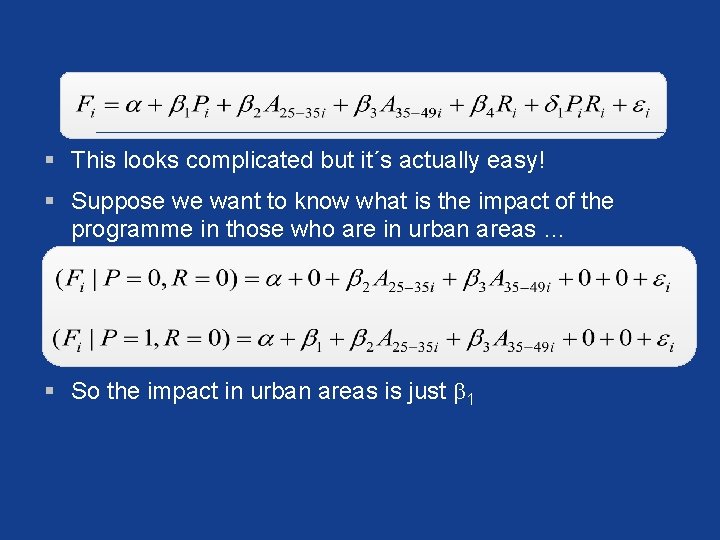
§ This looks complicated but it´s actually easy! § Suppose we want to know what is the impact of the programme in those who are in urban areas … § So the impact in urban areas is just b 1

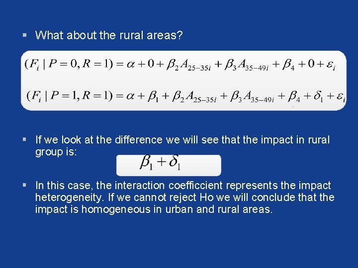
§ What about the rural areas? § If we look at the difference we will see that the impact in rural group is: § In this case, the interaction coefficcient represents the impact heterogeneity. If we cannot reject Ho we will conclude that the impact is homogeneous in urban and rural areas.

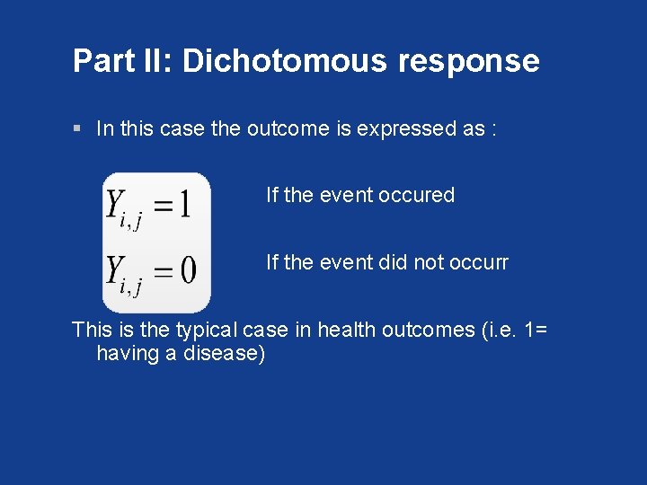
Part II: Dichotomous response § In this case the outcome is expressed as : If the event occured If the event did not occurr This is the typical case in health outcomes (i. e. 1= having a disease)

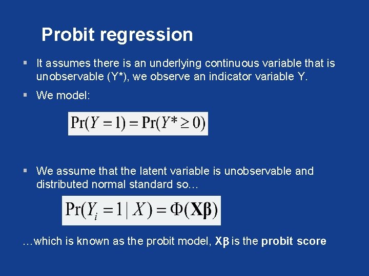
Probit regression § It assumes there is an underlying continuous variable that is unobservable (Y*), we observe an indicator variable Y. § We model: § We assume that the latent variable is unobservable and distributed normal standard so… …which is known as the probit model, Xb is the probit score

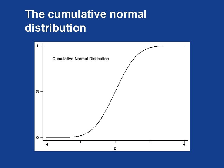
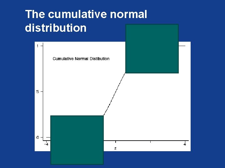
The cumulative normal distribution

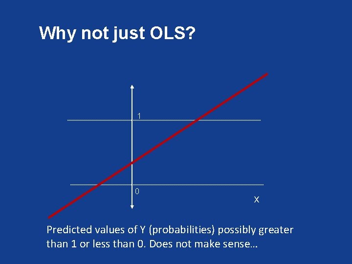
Why not just OLS? 1 0 X Predicted values of Y (probabilities) possibly greater than 1 or less than 0. Does not make sense…

§ The problem is b coefficients do not give you the marginal change in probability but the marginal change in the z-score!

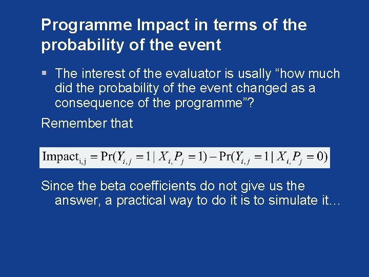
Programme Impact in terms of the probability of the event § The interest of the evaluator is usally “how much did the probability of the event changed as a consequence of the programme”? Remember that Since the beta coefficients do not give us the answer, a practical way to do it is to simulate it…

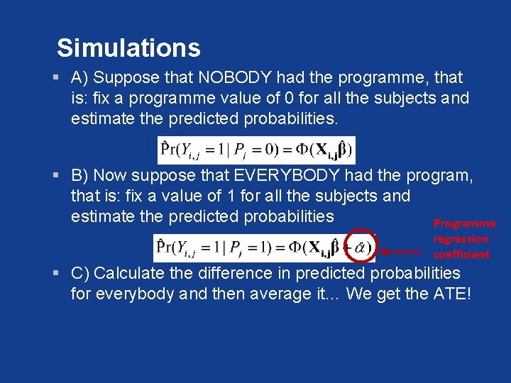
Simulations § A) Suppose that NOBODY had the programme, that is: fix a programme value of 0 for all the subjects and estimate the predicted probabilities. § B) Now suppose that EVERYBODY had the program, that is: fix a value of 1 for all the subjects and estimate the predicted probabilities Programme regression coefficient § C) Calculate the difference in predicted probabilities for everybody and then average it… We get the ATE!

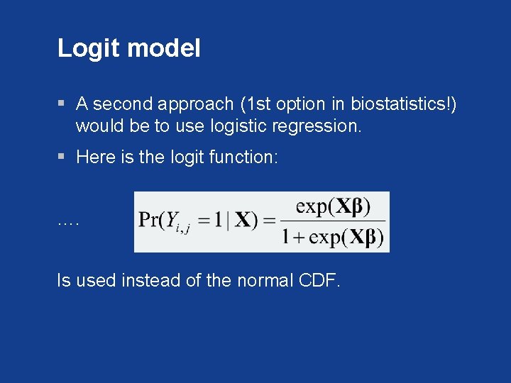
Logit model § A second approach (1 st option in biostatistics!) would be to use logistic regression. § Here is the logit function: …. Is used instead of the normal CDF.

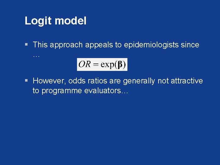
Logit model § This approach appeals to epidemiologists since … § However, odds ratios are generally not attractive to programme evaluators…

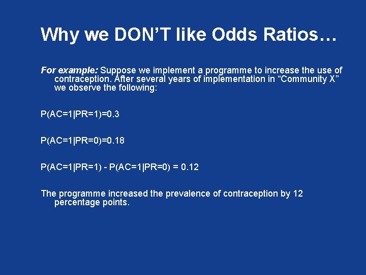
Why we DON’T like Odds Ratios… For example: Suppose we implement a programme to increase the use of contraception. After several years of implementation in “Community X” we observe the following: P(AC=1|PR=1)=0. 3 P(AC=1|PR=0)=0. 18 P(AC=1|PR=1) - P(AC=1|PR=0) = 0. 12 The programme increased the prevalence of contraception by 12 percentage points.

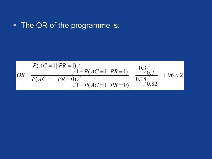
§ The OR of the programme is:

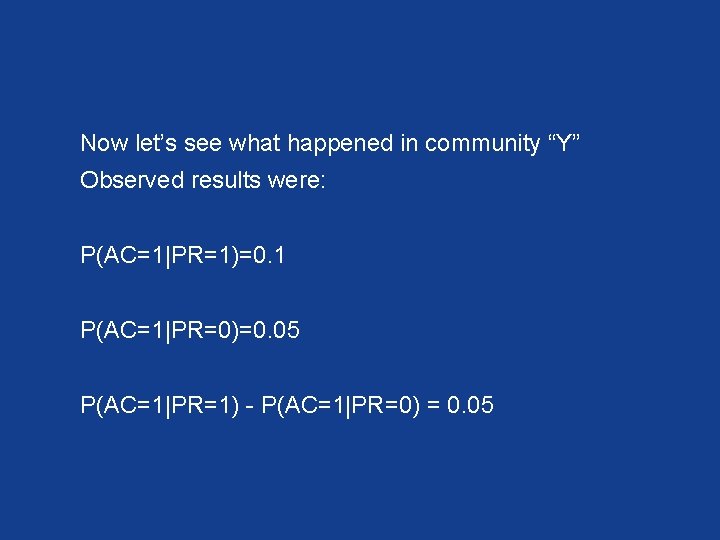
Now let’s see what happened in community “Y” Observed results were: P(AC=1|PR=1)=0. 1 P(AC=1|PR=0)=0. 05 P(AC=1|PR=1) - P(AC=1|PR=0) = 0. 05

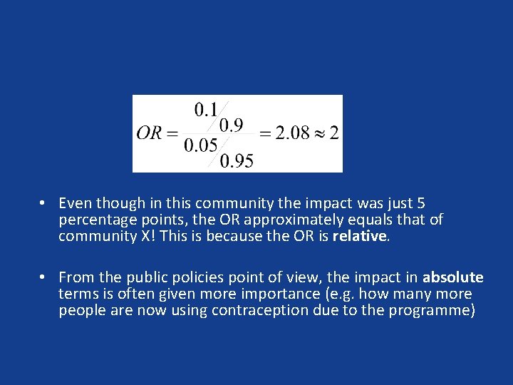
• Even though in this community the impact was just 5 percentage points, the OR approximately equals that of community X! This is because the OR is relative. • From the public policies point of view, the impact in absolute terms is often given more importance (e. g. how many more people are now using contraception due to the programme)

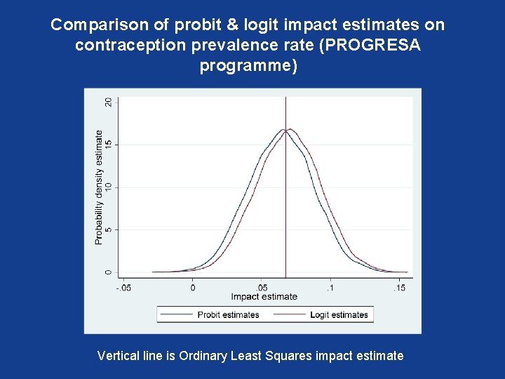
Comparison of probit & logit impact estimates on contraception prevalence rate (PROGRESA programme) Vertical line is Ordinary Least Squares impact estimate

Linear probability model § A third option would be to fit a OLS regression model even if the outcome is dichotomous. § Advantage: the b estimates directly tell us about the change in probability. No tricks are needed! § Disadvantage: Two assumptions: normality and homoscedasticity do not hold, however… § If the sample size is large, the estimates of E(Y|X) (in this case the probability of the event given X) will approximate a normal distribution (central limit theorem), specially when Pr(Y=1) approaches 0. 5 § We can use robust standard errors to account for heteroskedasticity.

The cumulative normal distribution

Extensions. . . Polytomous response § Sometimes the outcome variable is not dichotomous but has several categories. § These categories can either be ordered or not. § If ordered: § Ordinal models § Else: § Multinomial models

Ordered logit § It is an extension of the typical (dichotomous response) logit model. § Example of ordinal outcome: § Perceived health status: § Poor § Good § Excellent § Often, people use multinomial models for these outcomes, however it can not be recommended since: § We are ignoring important information! Categories are ordered, if we do, we will get inefficient impact estimates.

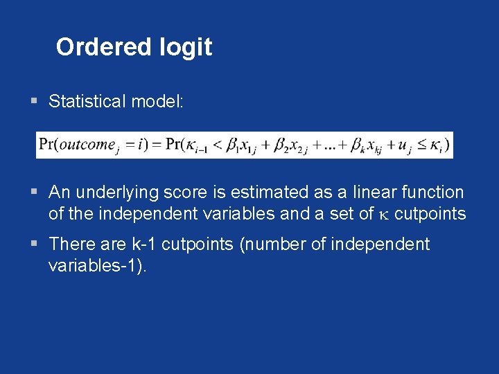
Ordered logit § Statistical model: § An underlying score is estimated as a linear function of the independent variables and a set of k cutpoints § There are k-1 cutpoints (number of independent variables-1).

Ordered logit § In this kind of models, the program impact would be measured as the probability increase (or decrease) in each particular value of the outcome.

Multinomial response § It could be that the outcome, has different categories that don’t really have an order: § Example of unordered outcome variable: § Use of contraceptive methods: § None § Natural methods § Barrier methods § Hormone-based methods

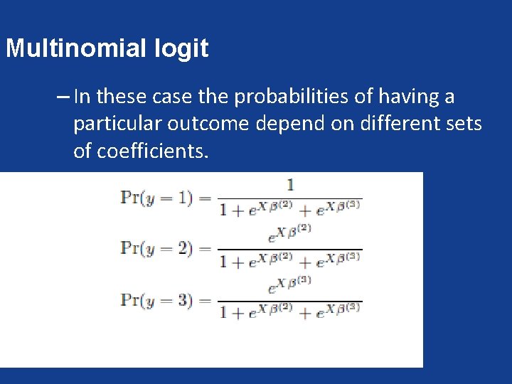
Multinomial logit – In these case the probabilities of having a particular outcome depend on different sets of coefficients.

Multinomial logit § Interpretation is the same as in the ordered case. § In both cases, simulations could be used to estimate the program effect. § There also Ordinal & Multinomial Probit models