Basic Parallel Computing Techniques Examples Problems with a

Basic Parallel Computing Techniques & Examples • Problems with a very large degree of (data) parallelism: (PP ch. 3) – Image Transformations: (also PP ch. 11) • Shifting, Rotation, Clipping etc. – Mandelbrot Set: • Sequential, static assignment, dynamic work pool assignment. • Divide-and-conquer Problem Partitioning: (pp ch. 4) – Parallel Bucket Sort – Numerical Integration: • Trapezoidal method using static assignment. • Adaptive Quadrature using dynamic assignment. – Gravitational N-Body Problem: Barnes-Hut Algorithm. • Pipelined Computation (pp ch. 5) – Pipelined Addition – Pipelined Insertion Sort – Pipelined Solution of A Set of Upper-Triangular Linear Equations Parallel Programming book, Chapters 3 -7, 11 EECC 756 - Shaaban #1 lec # 8 Spring 2003 4 -15 -2003

Basic Parallel Computing Techniques & Examples • Synchronous Iteration (Synchronous Parallelism) : (PP ch. 6) – Barriers: • Counter Barrier Implementation. • Tree Barrier Implementation. • Butterfly Connection Pattern Message-Passing Barrier. – Synchronous Iteration Program Example: • Iterative Solution of Linear Equations. • Dynamic Load Balancing (PP ch. 7) – Centralized Dynamic Load Balancing. – Decentralized Dynamic Load Balancing: • Distributed Work Pool Using Divide And Conquer. • Distributed Work Pool With Local Queues In Slaves. • Termination Detection for Decentralized Dynamic Load Balancing. – Program Example: Shortest Path Problem. EECC 756 - Shaaban #2 lec # 8 Spring 2003 4 -15 -2003

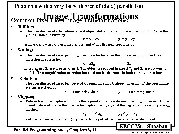
Problems with a very large degree of (data) parallelism Image Transformations Common Pixel-Level Transformations: • Shifting: • Scaling: • • – The coordinates of a two-dimensional object shifted by Dx in the x-direction and Dy in the y-dimension are given by: x' = x + Dx y' = y + Dy where x and y are the original, and x' and y' are the new coordinates. – The coordinates of an object magnified by a factor Sx in the x direction and Sy in the y direction are given by: x' = x. Sx y' = y. Sy where Sx and Sy are greater than 1. The object is reduced in size if Sx and Sy are between 0 and 1. The magnification or reduction need not be the same in both x and y directions. Rotation: – The coordinates of an object rotated through an angle q about the origin of the coordinate system are given by: x' = x cos q + y sin q y' = - x sin q + y cos q Clipping: – Deletes from the displayed picture those points outside a defined rectangular area. If the lowest values of x, y in the area to be display are x 1, y 1, and the highest values of x, y are xh, yh, then: x 1 £ xh y 1 £ y£ yh needs to be true for the point (x, y) to be displayed, otherwise (x, y) is not displayed. Parallel Programming book, Chapters 3, 11 EECC 756 - Shaaban #3 lec # 8 Spring 2003 4 -15 -2003

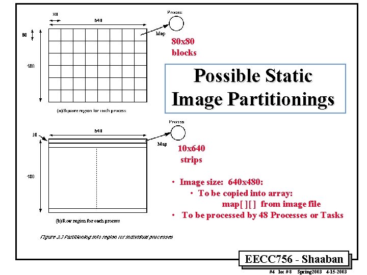
80 x 80 blocks Possible Static Image Partitionings 10 x 640 strips • Image size: 640 x 480: • To be copied into array: map[ ][ ] from image file • To be processed by 48 Processes or Tasks EECC 756 - Shaaban #4 lec # 8 Spring 2003 4 -15 -2003

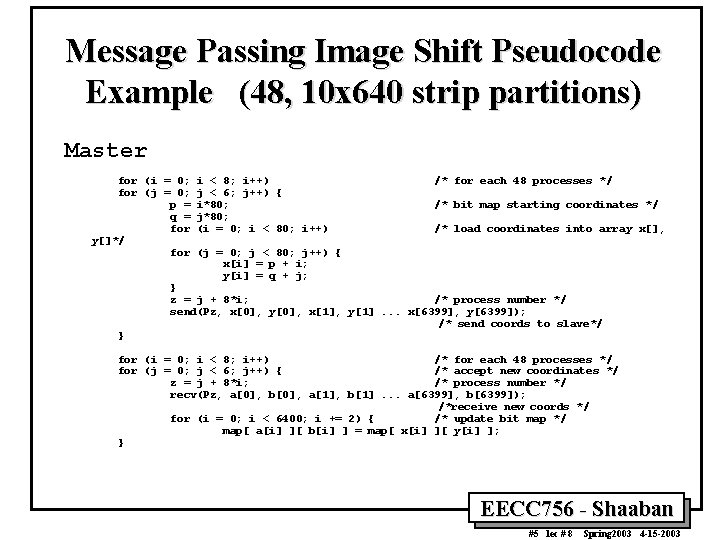
Message Passing Image Shift Pseudocode Example (48, 10 x 640 strip partitions) Master for (i = 0; i < 8; i++) /* for each 48 processes */ for (j = 0; j < 6; j++) { p = i*80; /* bit map starting coordinates */ q = j*80; for (i = 0; i < 80; i++) /* load coordinates into array x[], y[]*/ for (j = 0; j < 80; j++) { x[i] = p + i; y[i] = q + j; } z = j + 8*i; /* process number */ send(Pz, x[0], y[0], x[1], y[1]. . . x[6399], y[6399]); /* send coords to slave*/ } for (i = 0; i < 8; i++) /* for each 48 processes */ for (j = 0; j < 6; j++) { /* accept new coordinates */ z = j + 8*i; /* process number */ recv(Pz, a[0], b[0], a[1], b[1]. . . a[6399], b[6399]); /*receive new coords */ for (i = 0; i < 6400; i += 2) { /* update bit map */ map[ a[i] ][ b[i] ] = map[ x[i] ][ y[i] ]; } EECC 756 - Shaaban #5 lec # 8 Spring 2003 4 -15 -2003

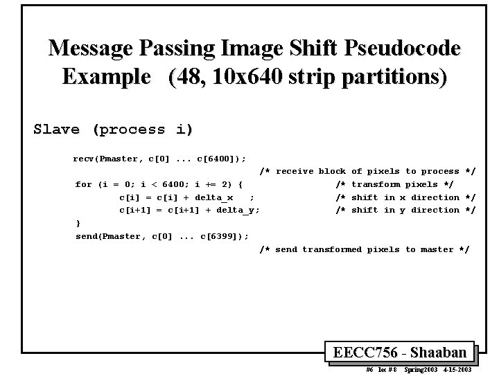
Message Passing Image Shift Pseudocode Example (48, 10 x 640 strip partitions) Slave (process i) recv(Pmaster, c[0]. . . c[6400]); /* receive block of pixels to process */ for (i = 0; i < 6400; i += 2) { /* transform pixels */ c[i] = c[i] + delta_x ; /* shift in x direction */ c[i+1] = c[i+1] + delta_y; /* shift in y direction */ } send(Pmaster, c[0]. . . c[6399]); /* send transformed pixels to master */ EECC 756 - Shaaban #6 lec # 8 Spring 2003 4 -15 -2003

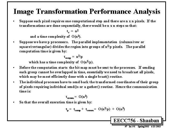
Image Transformation Performance Analysis • • • Suppose each pixel requires one computational step and there are n x n pixels. If the transformations are done sequentially, there would be n x n steps so that: ts = n 2 and a time complexity of O(n 2). Suppose we have p processors. The parallel implementation (column/row or square/rectangular) divides the region into groups of n 2/p pixels. The parallel computation time is given by: tcomp = n 2/p which has a time complexity of O(n 2/p). Before the computation starts the bit map must be sent to the processes. If sending each group cannot be overlapped in time, essentially we need to broadcast all pixels, which may be most efficiently done with a single bcast() routine. The individual processes have to send back the transformed coordinates of their group of pixels requiring individual send()s or a gather() routine. Hence the communication time is: tcomm = O(n 2) So that the overall execution time is given by: tp = tcomp + tcomm = O(n 2/p) + O(n 2) EECC 756 - Shaaban #7 lec # 8 Spring 2003 4 -15 -2003

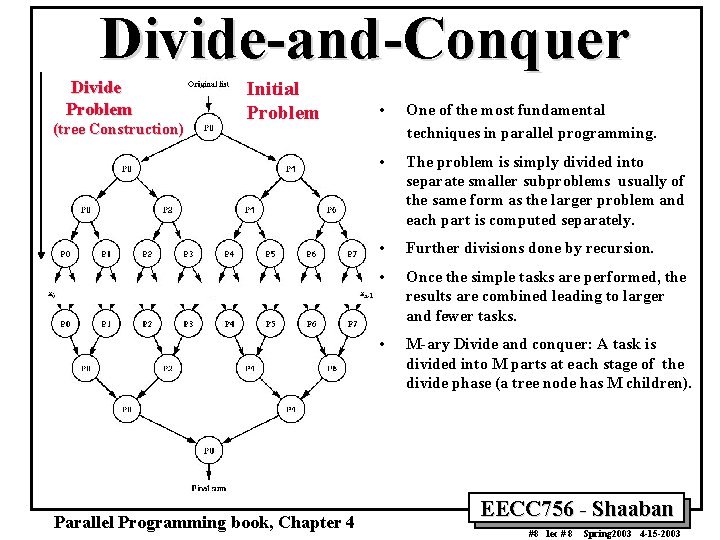
Divide-and-Conquer Divide Problem (tree Construction) Initial Problem Parallel Programming book, Chapter 4 • One of the most fundamental techniques in parallel programming. • The problem is simply divided into separate smaller subproblems usually of the same form as the larger problem and each part is computed separately. • Further divisions done by recursion. • Once the simple tasks are performed, the results are combined leading to larger and fewer tasks. • M-ary Divide and conquer: A task is divided into M parts at each stage of the divide phase (a tree node has M children). EECC 756 - Shaaban #8 lec # 8 Spring 2003 4 -15 -2003

Divide-and-Conquer Example Bucket Sort • On a sequential computer, it requires n steps to place the n numbers into m buckets (by dividing each number by m). • If the numbers are uniformly distributed, there should be about n/m numbers in each bucket. • Next the numbers in each bucket must be sorted: Sequential sorting algorithms such as Quicksort or Mergesort have a time complexity of O(nlog 2 n) to sort n numbers. • Then it will take typically (n/m)log 2(n/m) steps to sort the n/m numbers in each bucket using a sequential sorting algorithm such as Quicksort or Mergesort, leading to sequential time of: ts = n + m((n/m)log 2(n/m)) = n + nlog 2(n/m) = O(nlog 2(n/m)) • If n = km where k is a constant, we get a linear complexity of O(n). EECC 756 - Shaaban #9 lec # 8 Spring 2003 4 -15 -2003

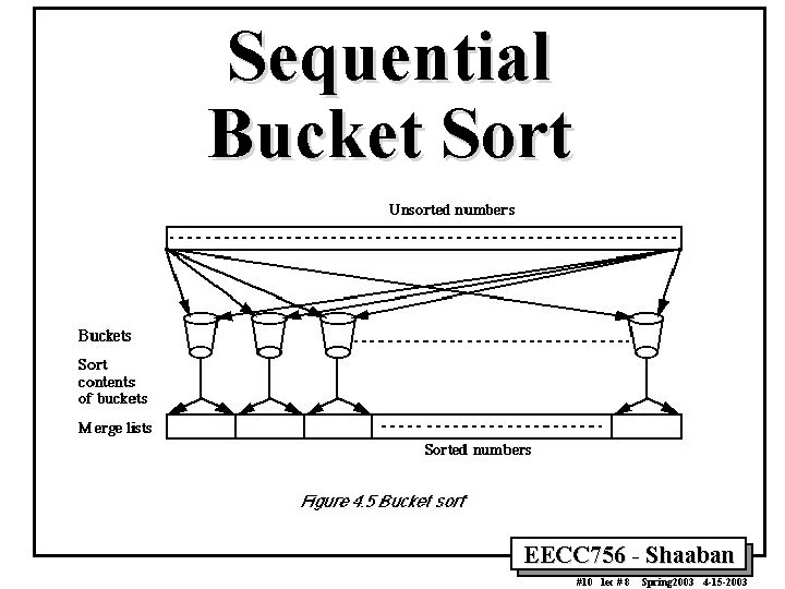
Sequential Bucket Sort EECC 756 - Shaaban #10 lec # 8 Spring 2003 4 -15 -2003

Parallel Bucket Sort • Bucket sort can be parallelized by assigning one processor for each bucket this reduces the sort time to (n/p)log(n/p) (m = p processors). • Can be further improved by having processors remove numbers from the list into their buckets, so that these numbers are not considered by other processors. • Can be further parallelized by partitioning the sequence into m regions, one region for each processor. • Each processor maintains p “small” buckets and separates the numbers in its region into its small buckets. • These small buckets are then emptied into the p final buckets for sorting, which requires each processor to send one small bucket to each of the other processors (bucket i to processor i). • Phases: – – Phase 1: Phase 2: Phase 3: Phase 4: Partition numbers among processors. Separate numbers into small buckets in each processor. Send to large buckets. Sort large buckets in each processor. EECC 756 - Shaaban #11 lec # 8 Spring 2003 4 -15 -2003

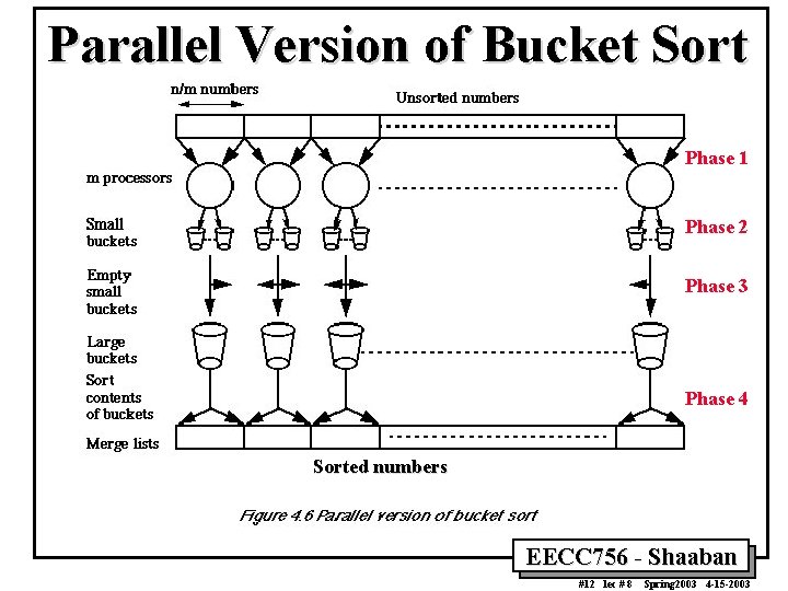
Parallel Version of Bucket Sort Phase 1 Phase 2 Phase 3 Phase 4 Sorted numbers EECC 756 - Shaaban #12 lec # 8 Spring 2003 4 -15 -2003

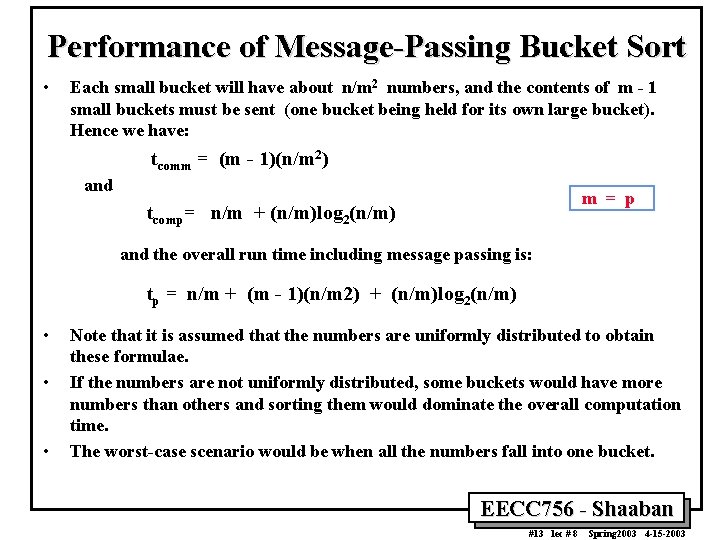
Performance of Message-Passing Bucket Sort • Each small bucket will have about n/m 2 numbers, and the contents of m - 1 small buckets must be sent (one bucket being held for its own large bucket). Hence we have: tcomm = (m - 1)(n/m 2) and m = p tcomp= n/m + (n/m)log 2(n/m) and the overall run time including message passing is: tp = n/m + (m - 1)(n/m 2) + (n/m)log 2(n/m) • • • Note that it is assumed that the numbers are uniformly distributed to obtain these formulae. If the numbers are not uniformly distributed, some buckets would have more numbers than others and sorting them would dominate the overall computation time. The worst-case scenario would be when all the numbers fall into one bucket. EECC 756 - Shaaban #13 lec # 8 Spring 2003 4 -15 -2003

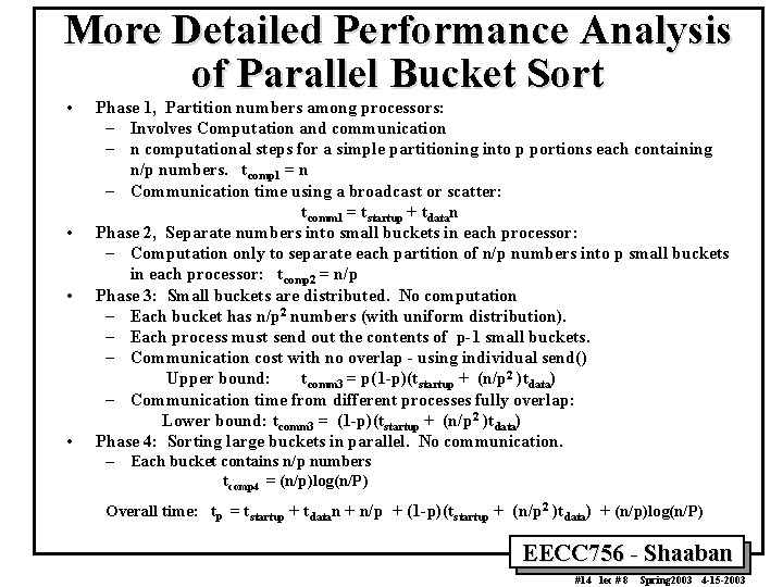
More Detailed Performance Analysis of Parallel Bucket Sort • • Phase 1, Partition numbers among processors: – Involves Computation and communication – n computational steps for a simple partitioning into p portions each containing n/p numbers. tcomp 1 = n – Communication time using a broadcast or scatter: tcomm 1 = tstartup + tdatan Phase 2, Separate numbers into small buckets in each processor: – Computation only to separate each partition of n/p numbers into p small buckets in each processor: tcomp 2 = n/p Phase 3: Small buckets are distributed. No computation – Each bucket has n/p 2 numbers (with uniform distribution). – Each process must send out the contents of p-1 small buckets. – Communication cost with no overlap - using individual send() Upper bound: tcomm 3 = p(1 -p)(tstartup + (n/p 2 )tdata) – Communication time from different processes fully overlap: Lower bound: tcomm 3 = (1 -p)(tstartup + (n/p 2 )tdata) Phase 4: Sorting large buckets in parallel. No communication. – Each bucket contains n/p numbers tcomp 4 = (n/p)log(n/P) Overall time: tp = tstartup + tdatan + n/p + (1 -p)(tstartup + (n/p 2 )tdata) + (n/p)log(n/P) EECC 756 - Shaaban #14 lec # 8 Spring 2003 4 -15 -2003

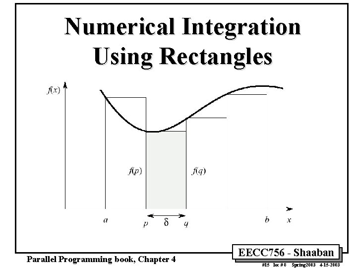
Numerical Integration Using Rectangles Parallel Programming book, Chapter 4 EECC 756 - Shaaban #15 lec # 8 Spring 2003 4 -15 -2003

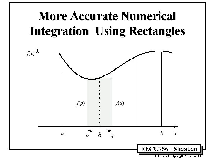
More Accurate Numerical Integration Using Rectangles EECC 756 - Shaaban #16 lec # 8 Spring 2003 4 -15 -2003

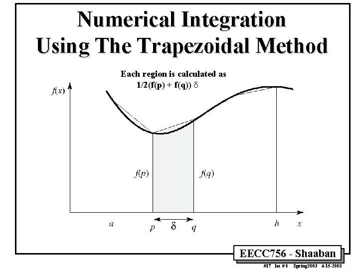
Numerical Integration Using The Trapezoidal Method Each region is calculated as 1/2(f(p) + f(q)) d EECC 756 - Shaaban #17 lec # 8 Spring 2003 4 -15 -2003

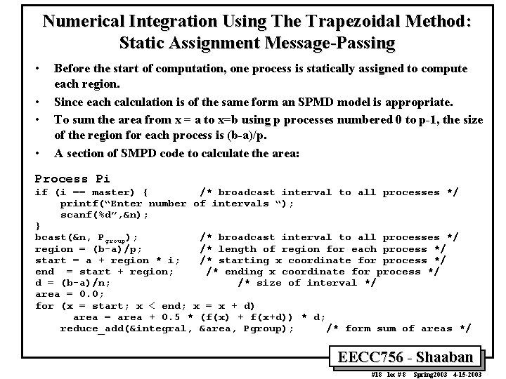
Numerical Integration Using The Trapezoidal Method: Static Assignment Message-Passing • • Before the start of computation, one process is statically assigned to compute each region. Since each calculation is of the same form an SPMD model is appropriate. To sum the area from x = a to x=b using p processes numbered 0 to p-1, the size of the region for each process is (b-a)/p. A section of SMPD code to calculate the area: Process Pi if (i == master) { /* broadcast interval to all processes */ printf(“Enter number of intervals “); scanf(%d”, &n); } bcast(&n, Pgroup); /* broadcast interval to all processes */ region = (b-a)/p; /* length of region for each process */ start = a + region * i; /* starting x coordinate for process */ end = start + region; /* ending x coordinate for process */ d = (b-a)/n; /* size of interval */ area = 0. 0; for (x = start; x < end; x = x + d) area = area + 0. 5 * (f(x) + f(x+d)) * d; reduce_add(&integral, &area, Pgroup); /* form sum of areas */ EECC 756 - Shaaban #18 lec # 8 Spring 2003 4 -15 -2003

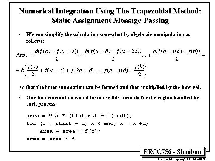
Numerical Integration Using The Trapezoidal Method: Static Assignment Message-Passing • We can simplify the calculation somewhat by algebraic manipulation as follows: so that the inner summation can be formed and then multiplied by the interval. • One implementation would be to use this formula for the region handled by each process: area = 0. 5 * (f(start) + f(end)); for (x = start + d; x < end; x = x +d) area = area + f(x); area = area * d EECC 756 - Shaaban #19 lec # 8 Spring 2003 4 -15 -2003

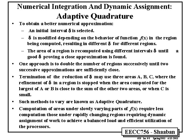
Numerical Integration And Dynamic Assignment: • • • Adaptive Quadrature To obtain a better numerical approximation: – An initial interval d is selected. – d is modified depending on the behavior of function f(x) in the region being computed, resulting in different d for different regions. – The area of a region is recomputed using different intervals d until a good d proving a close approximation is found. One approach is to double the number of regions successively until two successive approximations are sufficiently close. Termination of the reduction of d may use three areas A, B, C, where the refinement of d in a region is stopped when the area computed for the largest of A or B is close to the sum of the other two areas, or when C is small. Such methods to vary are known as Adaptive Quadrature. Computation of areas under slowly varying parts of f(x) require less computation those under rapidly changing regions requiring dynamic assignment of work to achieve a balanced load and efficient utilization of the processors. EECC 756 - Shaaban #20 lec # 8 Spring 2003 4 -15 -2003

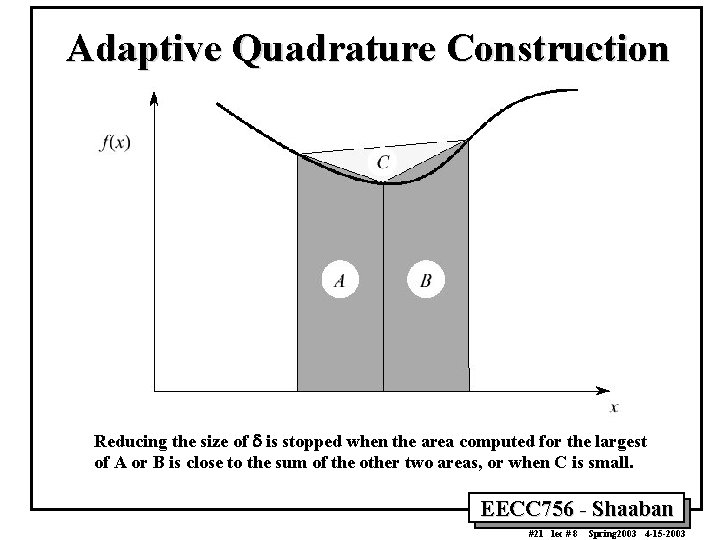
Adaptive Quadrature Construction Reducing the size of d is stopped when the area computed for the largest of A or B is close to the sum of the other two areas, or when C is small. EECC 756 - Shaaban #21 lec # 8 Spring 2003 4 -15 -2003

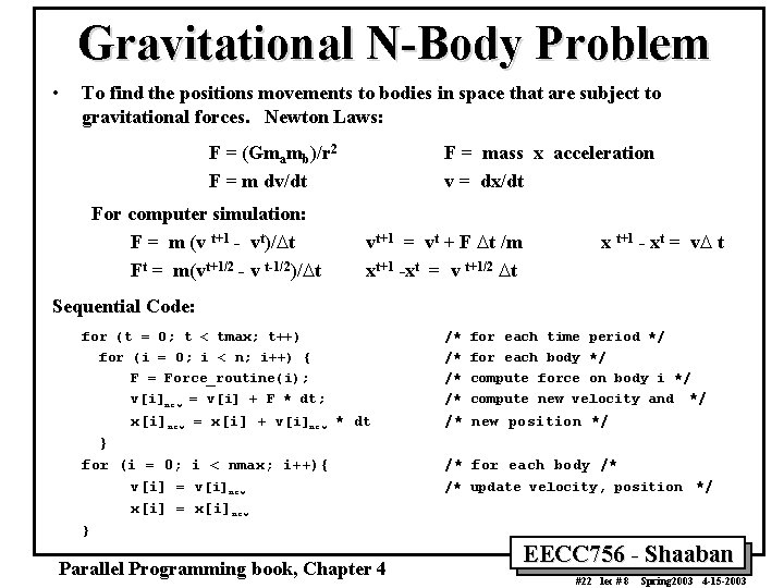
Gravitational N-Body Problem • To find the positions movements to bodies in space that are subject to gravitational forces. Newton Laws: F = (Gmamb)/r 2 F = m dv/dt For computer simulation: F = m (v t+1 - vt)/Dt Ft = m(vt+1/2 - v t-1/2)/Dt F = mass x acceleration v = dx/dt vt+1 = vt + F Dt /m xt+1 -xt = v t+1/2 Dt x t+1 - xt = v. D t Sequential Code: for (t = 0; t < tmax; t++) for (i = 0; i < n; i++) { F = Force_routine(i); /* for each time period */ /* for each body */ /* compute force on body i */ v[i]new = v[i] + F * dt; /* compute new velocity and x[i]new = x[i] + v[i]new * dt /* new position */ } for (i = 0; i < nmax; i++){ v[i] = v[i]new x[i] = x[i]new */ /* for each body /* /* update velocity, position */ } Parallel Programming book, Chapter 4 EECC 756 - Shaaban #22 lec # 8 Spring 2003 4 -15 -2003

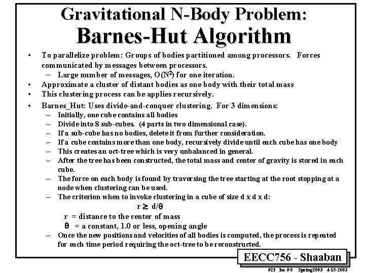
Gravitational N-Body Problem: Barnes-Hut Algorithm • • To parallelize problem: Groups of bodies partitioned among processors. Forces communicated by messages between processors. – Large number of messages, O(N 2) for one iteration. Approximate a cluster of distant bodies as one body with their total mass This clustering process can be applies recursively. Barnes_Hut: Uses divide-and-conquer clustering. For 3 dimensions: – Initially, one cube contains all bodies – Divide into 8 sub-cubes. (4 parts in two dimensional case). – If a sub-cube has no bodies, delete it from further consideration. – If a cube contains more than one body, recursively divide until each cube has one body – This creates an oct-tree which is very unbalanced in general. – After the tree has been constructed, the total mass and center of gravity is stored in each cube. – The force on each body is found by traversing the tree starting at the root stopping at a node when clustering can be used. – The criterion when to invoke clustering in a cube of size d x d: r ³ d/q r = distance to the center of mass q = a constant, 1. 0 or less, opening angle – Once the new positions and velocities of all bodies is computed, the process is repeated for each time period requiring the oct-tree to be reconstructed. EECC 756 - Shaaban #23 lec # 8 Spring 2003 4 -15 -2003

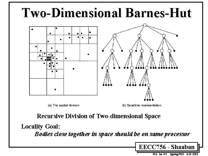
Two-Dimensional Barnes-Hut Recursive Division of Two-dimensional Space Locality Goal: Bodies close together in space should be on same processor EECC 756 - Shaaban #24 lec # 8 Spring 2003 4 -15 -2003

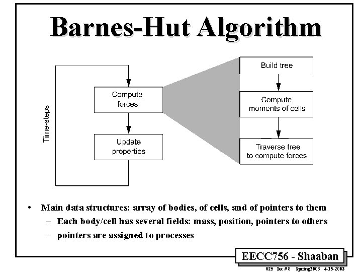
Barnes-Hut Algorithm • Main data structures: array of bodies, of cells, and of pointers to them – Each body/cell has several fields: mass, position, pointers to others – pointers are assigned to processes EECC 756 - Shaaban #25 lec # 8 Spring 2003 4 -15 -2003

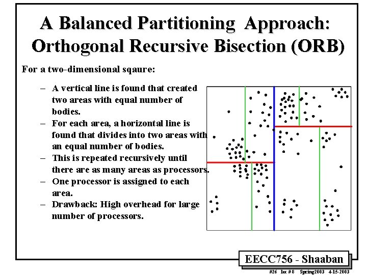
A Balanced Partitioning Approach: Orthogonal Recursive Bisection (ORB) For a two-dimensional sqaure: – A vertical line is found that created two areas with equal number of bodies. – For each area, a horizontal line is found that divides into two areas with an equal number of bodies. – This is repeated recursively until there as many areas as processors. – One processor is assigned to each area. – Drawback: High overhead for large number of processors. EECC 756 - Shaaban #26 lec # 8 Spring 2003 4 -15 -2003

Pipelined Computations • Given the problem can be divided into a series of sequential operations, the pipelined approach can provide increase speed under any of the following three "types" of computations: 1. If more than one instance of the complete problem is to be executed. 2. A series of data items must be processed with multiple operations. 3. If information to start the next process can be passed forward before the process has completed all its internal operations. Parallel Programming book, Chapter 5 EECC 756 - Shaaban #27 lec # 8 Spring 2003 4 -15 -2003

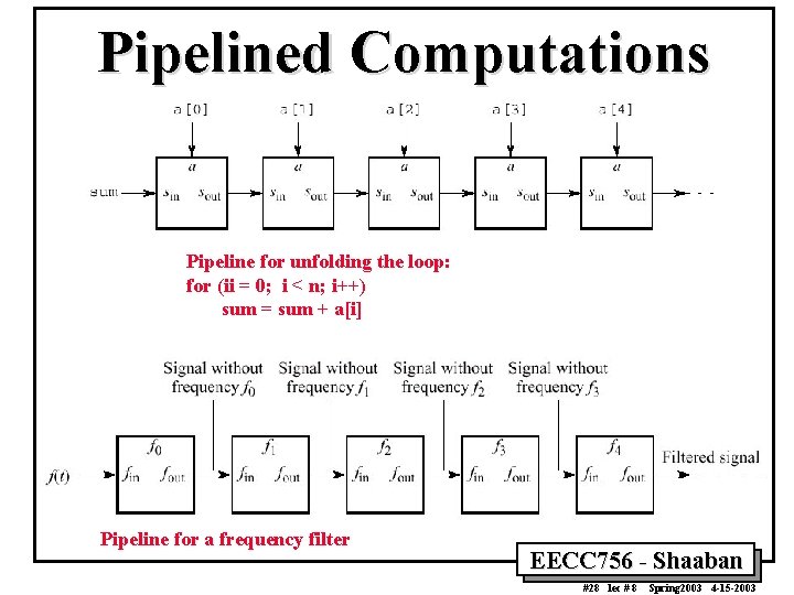
Pipelined Computations Pipeline for unfolding the loop: for (ii = 0; i < n; i++) sum = sum + a[i] Pipeline for a frequency filter EECC 756 - Shaaban #28 lec # 8 Spring 2003 4 -15 -2003

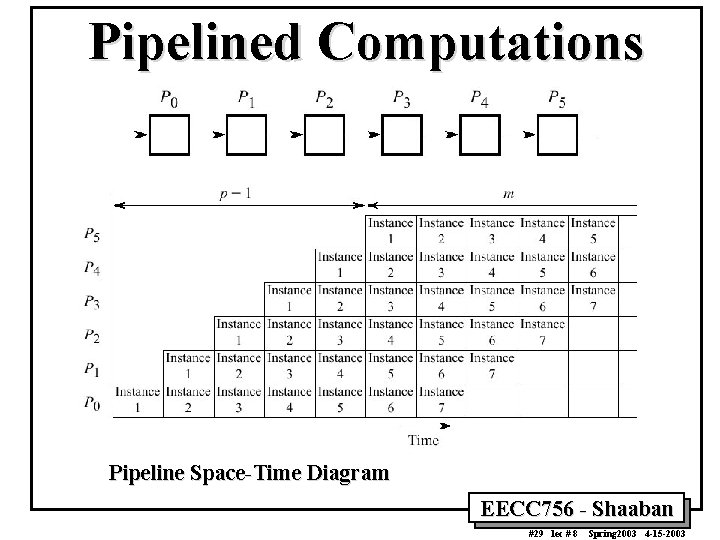
Pipelined Computations Pipeline Space-Time Diagram EECC 756 - Shaaban #29 lec # 8 Spring 2003 4 -15 -2003

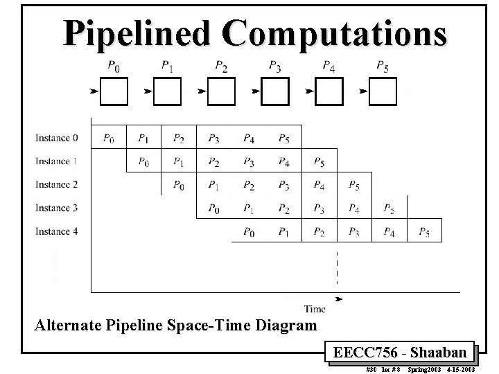
Pipelined Computations Alternate Pipeline Space-Time Diagram EECC 756 - Shaaban #30 lec # 8 Spring 2003 4 -15 -2003

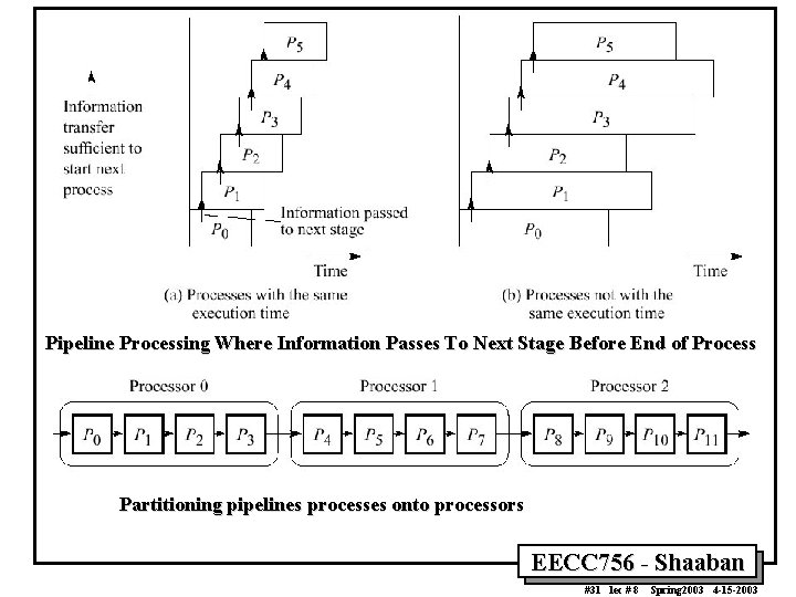
Pipeline Processing Where Information Passes To Next Stage Before End of Process Partitioning pipelines processes onto processors EECC 756 - Shaaban #31 lec # 8 Spring 2003 4 -15 -2003

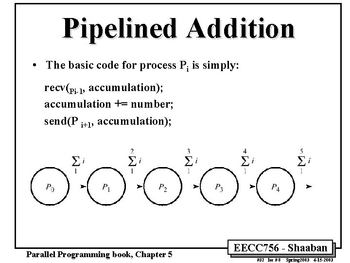
Pipelined Addition • The basic code for process Pi is simply: recv(Pi-1, accumulation); accumulation += number; send(P i+1, accumulation); Parallel Programming book, Chapter 5 EECC 756 - Shaaban #32 lec # 8 Spring 2003 4 -15 -2003

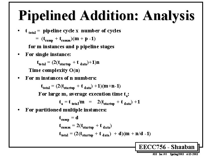
Pipelined Addition: Analysis • • t total = pipeline cycle x number of cycles = (tcomp + tcomm)(m + p -1) for m instances and p pipeline stages For single instance: ttotal = (2(tstartup + t data)+1)n Time complexity O(n) For m instances of n numbers: ttotal = (2(tstartup + t data) +1)(m+n-1) For large m, average execution time ta: ta = t total/m = 2(tstartup + t data) +1 For partitioned multiple instances: tcomp = d tcomm = 2(tstartup + t data) ttotal = (2(tstartup + t data) + d)(m + n/d -1) EECC 756 - Shaaban #33 lec # 8 Spring 2003 4 -15 -2003

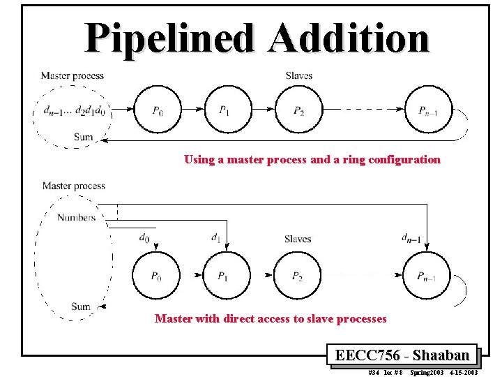
Pipelined Addition Using a master process and a ring configuration Master with direct access to slave processes EECC 756 - Shaaban #34 lec # 8 Spring 2003 4 -15 -2003

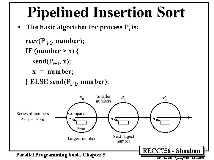
Pipelined Insertion Sort • The basic algorithm for process Pi is: recv(P i-1, number); IF (number > x) { send(Pi+1, x); x = number; } ELSE send(Pi+1, number); Parallel Programming book, Chapter 5 EECC 756 - Shaaban #35 lec # 8 Spring 2003 4 -15 -2003

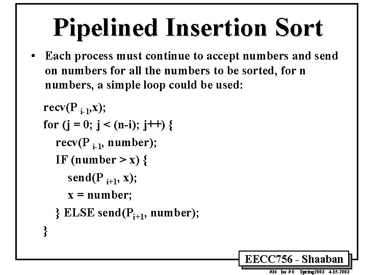
Pipelined Insertion Sort • Each process must continue to accept numbers and send on numbers for all the numbers to be sorted, for n numbers, a simple loop could be used: recv(P i-1, x); for (j = 0; j < (n-i); j++) { recv(P i-1, number); IF (number > x) { send(P i+1, x); x = number; } ELSE send(Pi+1, number); } EECC 756 - Shaaban #36 lec # 8 Spring 2003 4 -15 -2003

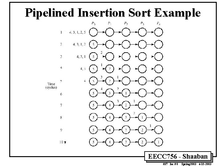
Pipelined Insertion Sort Example EECC 756 - Shaaban #37 lec # 8 Spring 2003 4 -15 -2003

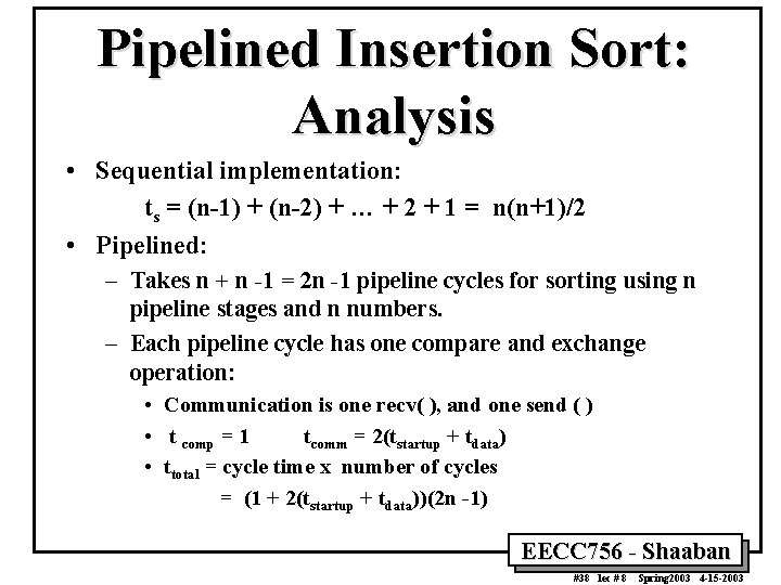
Pipelined Insertion Sort: Analysis • Sequential implementation: ts = (n-1) + (n-2) + … + 2 + 1 = n(n+1)/2 • Pipelined: – Takes n + n -1 = 2 n -1 pipeline cycles for sorting using n pipeline stages and n numbers. – Each pipeline cycle has one compare and exchange operation: • Communication is one recv( ), and one send ( ) • t comp = 1 tcomm = 2(tstartup + tdata) • ttotal = cycle time x number of cycles = (1 + 2(tstartup + tdata))(2 n -1) EECC 756 - Shaaban #38 lec # 8 Spring 2003 4 -15 -2003

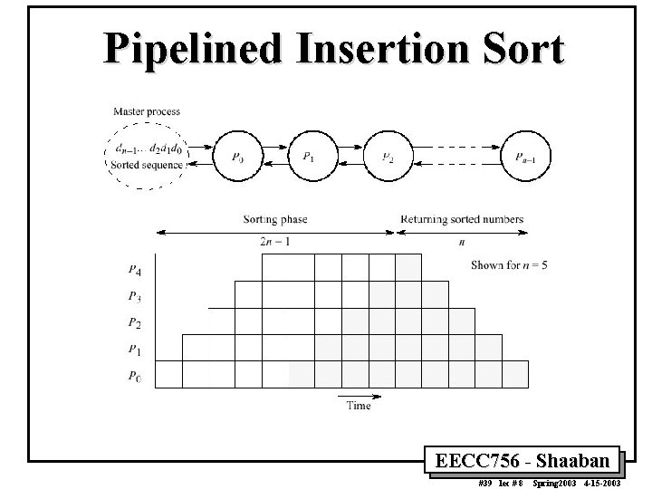
Pipelined Insertion Sort EECC 756 - Shaaban #39 lec # 8 Spring 2003 4 -15 -2003

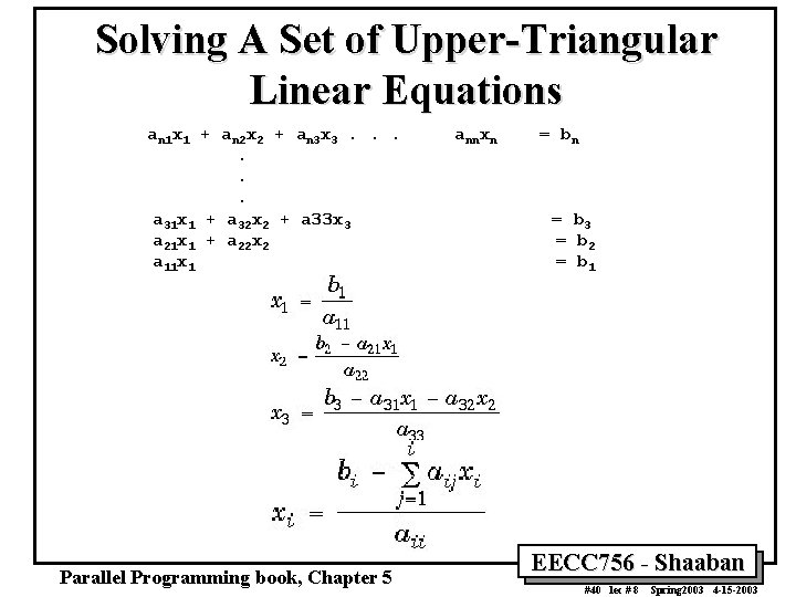
Solving A Set of Upper-Triangular Linear Equations an 1 x 1 + an 2 x 2 + an 3 x 3. . . a 31 x 1 + a 32 x 2 + a 33 x 3 a 21 x 1 + a 22 x 2 a 11 x 1 Parallel Programming book, Chapter 5 annxn = b 3 = b 2 = b 1 EECC 756 - Shaaban #40 lec # 8 Spring 2003 4 -15 -2003

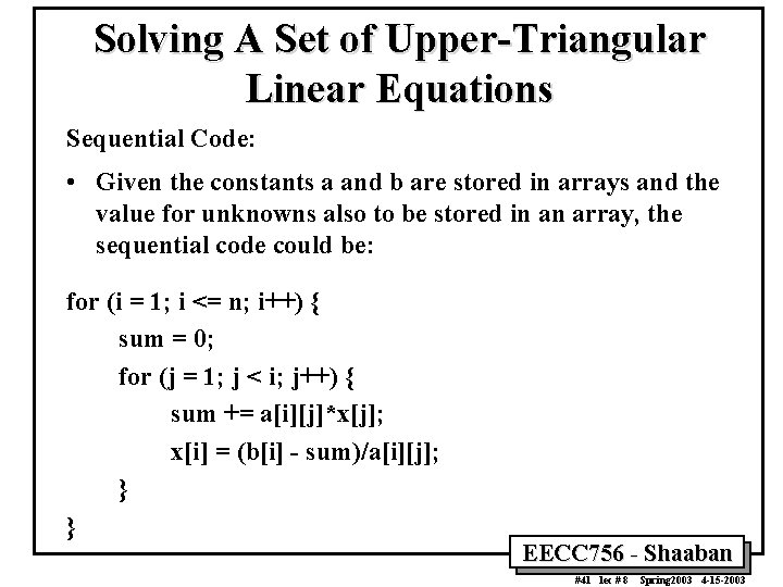
Solving A Set of Upper-Triangular Linear Equations Sequential Code: • Given the constants a and b are stored in arrays and the value for unknowns also to be stored in an array, the sequential code could be: for (i = 1; i <= n; i++) { sum = 0; for (j = 1; j < i; j++) { sum += a[i][j]*x[j]; x[i] = (b[i] - sum)/a[i][j]; } } EECC 756 - Shaaban #41 lec # 8 Spring 2003 4 -15 -2003

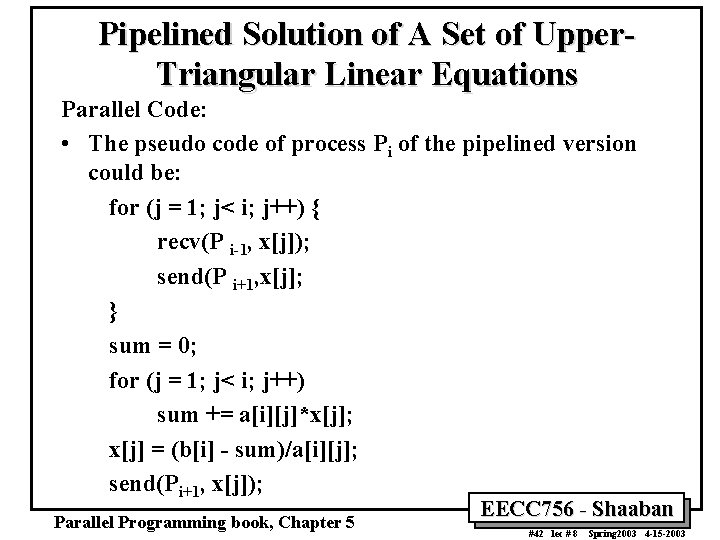
Pipelined Solution of A Set of Upper. Triangular Linear Equations Parallel Code: • The pseudo code of process Pi of the pipelined version could be: for (j = 1; j< i; j++) { recv(P i-1, x[j]); send(P i+1, x[j]; } sum = 0; for (j = 1; j< i; j++) sum += a[i][j]*x[j]; x[j] = (b[i] - sum)/a[i][j]; send(Pi+1, x[j]); Parallel Programming book, Chapter 5 EECC 756 - Shaaban #42 lec # 8 Spring 2003 4 -15 -2003

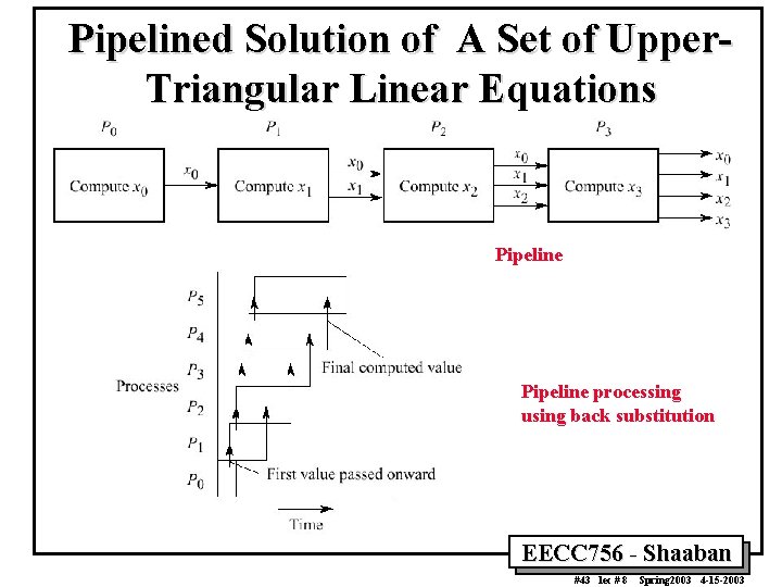
Pipelined Solution of A Set of Upper. Triangular Linear Equations Pipeline processing using back substitution EECC 756 - Shaaban #43 lec # 8 Spring 2003 4 -15 -2003

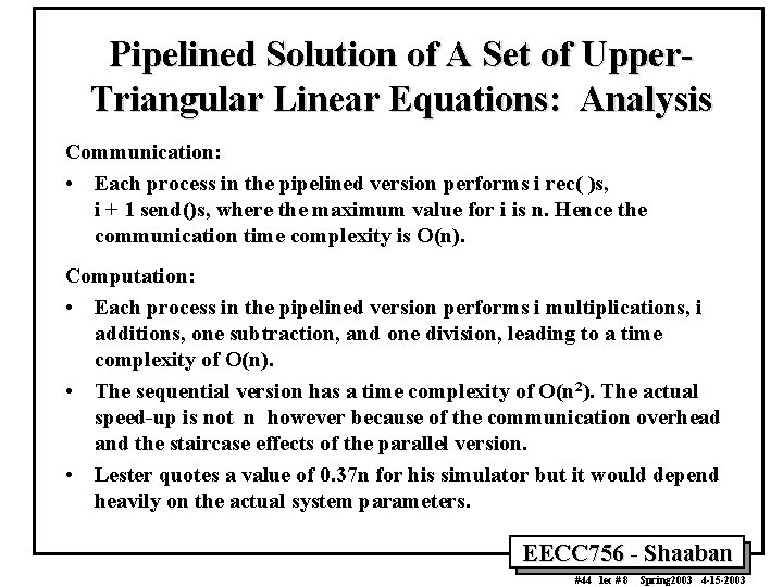
Pipelined Solution of A Set of Upper. Triangular Linear Equations: Analysis Communication: • Each process in the pipelined version performs i rec( )s, i + 1 send()s, where the maximum value for i is n. Hence the communication time complexity is O(n). Computation: • Each process in the pipelined version performs i multiplications, i additions, one subtraction, and one division, leading to a time complexity of O(n). • The sequential version has a time complexity of O(n 2). The actual speed-up is not n however because of the communication overhead and the staircase effects of the parallel version. • Lester quotes a value of 0. 37 n for his simulator but it would depend heavily on the actual system parameters. EECC 756 - Shaaban #44 lec # 8 Spring 2003 4 -15 -2003

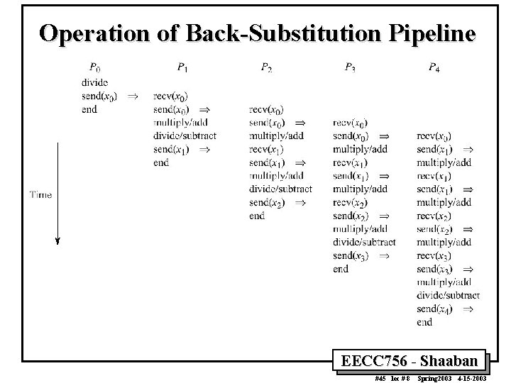
Operation of Back-Substitution Pipeline EECC 756 - Shaaban #45 lec # 8 Spring 2003 4 -15 -2003

Synchronous Iteration • Iteration-based computation is a powerful method for solving numerical (and some non-numerical) problems. • For numerical problems, a calculation is repeated and each time, a result is obtained which is used on the next execution. The process is repeated until the desired results are obtained. • Though iterative methods are is sequential in nature, parallel implementation can be successfully employed when there are multiple independent instances of the iteration. In some cases this is part of the problem specification and sometimes one must rearrange the problem to obtain multiple independent instances. • The term "synchronous iteration" is used to describe solving a problem by iteration where different tasks may be performing separate iterations but the iterations must be synchronized using point-to-point synchronization, barriers, or other synchronization mechanisms. Parallel Programming book, Chapter 6 EECC 756 - Shaaban #46 lec # 8 Spring 2003 4 -15 -2003

Synchronous Iteration (Synchronous Parallelism) • Each iteration composed of several processes that start together at beginning of iteration. Next iteration cannot begin until all processes have finished previous iteration. Using forall : for (j = 0; j < n; j++) /*for each synch. iteration */ forall (i = 0; i < N; i++) { /*N processes each using*/ body(i); /* specific value of i */ } • or: for (j = 0; j < n; j++) { /*for each synchr. iteration */ i = myrank; /*find value of i to be used */ body(i); barrier(mygroup); } EECC 756 - Shaaban #47 lec # 8 Spring 2003 4 -15 -2003

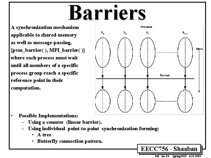
Barriers A synchronization mechanism applicable to shared-memory as well as message-passing, [pvm_barrier( ), MPI_barrier( )] where each process must wait until all members of a specific process group reach a specific reference point in their computation. • Possible Implementations: – Using a counter (linear barrier). – Using individual point-to-point synchronization forming: • A tree • Butterfly connection pattern. EECC 756 - Shaaban #48 lec # 8 Spring 2003 4 -15 -2003

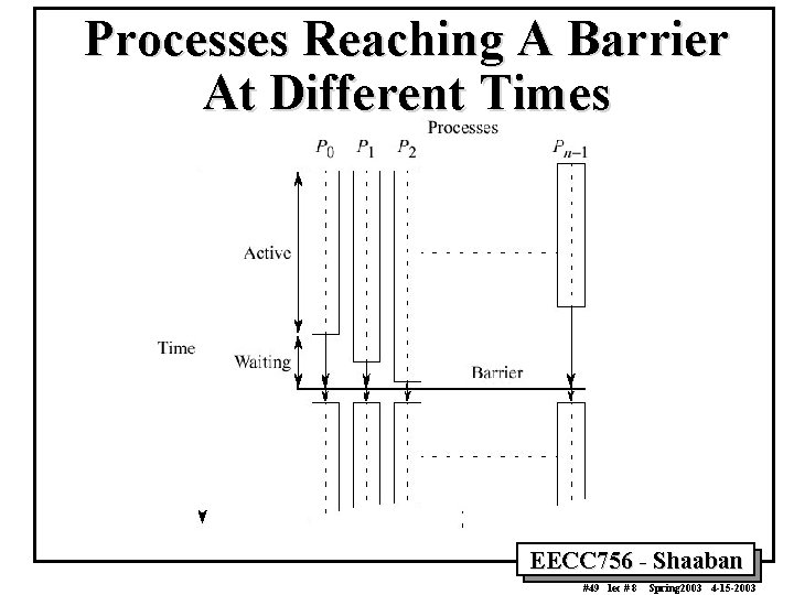
Processes Reaching A Barrier At Different Times EECC 756 - Shaaban #49 lec # 8 Spring 2003 4 -15 -2003

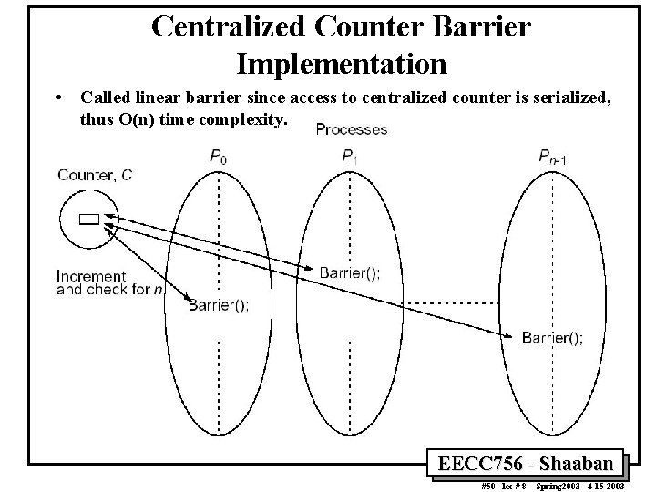
Centralized Counter Barrier Implementation • Called linear barrier since access to centralized counter is serialized, thus O(n) time complexity. EECC 756 - Shaaban #50 lec # 8 Spring 2003 4 -15 -2003

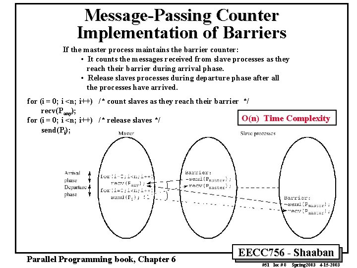
Message-Passing Counter Implementation of Barriers If the master process maintains the barrier counter: • It counts the messages received from slave processes as they reach their barrier during arrival phase. • Release slaves processes during departure phase after all the processes have arrived. for (i = 0; i <n; i++) /* count slaves as they reach their barrier */ recv(Pany); O(n) Time Complexity for (i = 0; i <n; i++) /* release slaves */ send(Pi); Parallel Programming book, Chapter 6 EECC 756 - Shaaban #51 lec # 8 Spring 2003 4 -15 -2003

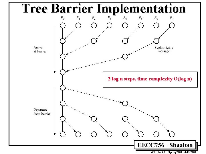
Tree Barrier Implementation 2 log n steps, time complexity O(log n) EECC 756 - Shaaban #52 lec # 8 Spring 2003 4 -15 -2003

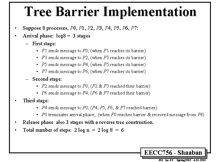
Tree Barrier Implementation • • Suppose 8 processes, P 0, P 1, P 2, P 3, P 4, P 5, P 6, P 7: Arrival phase: log 8 = 3 stages – First stage: • • P 1 sends message to P 0; (when P 1 reaches its barrier) P 3 sends message to P 2; (when P 3 reaches its barrier) P 5 sends message to P 4; (when P 5 reaches its barrier) P 7 sends message to P 6; (when P 7 reaches its barrier) – Second stage: • P 2 sends message to P 0; (P 2 & P 3 reached their barrier) • P 6 sends message to P 4; (P 6 & P 7 reached their barrier) • Third stage: • P 4 sends message to P 0; (P 4, P 5, P 6, & P 7 reached barrier) • P 0 terminates arrival phase; (when P 0 reaches barrier & received message from P 4) • • Release phase also 3 stages with a reverse tree construction. Total number of steps: 2 log n = 2 log 8 = 6 EECC 756 - Shaaban #53 lec # 8 Spring 2003 4 -15 -2003

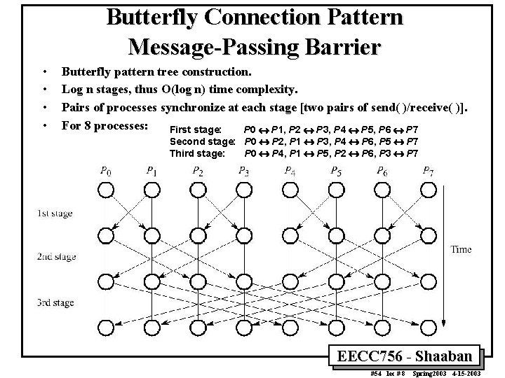
Butterfly Connection Pattern Message-Passing Barrier • • Butterfly pattern tree construction. Log n stages, thus O(log n) time complexity. Pairs of processes synchronize at each stage [two pairs of send( )/receive( )]. For 8 processes: First stage: P 0 « P 1, P 2 « P 3, P 4 « P 5, P 6 « P 7 Second stage: P 0 « P 2, P 1 « P 3, P 4 « P 6, P 5 « P 7 Third stage: P 0 « P 4, P 1 « P 5, P 2 « P 6, P 3 « P 7 EECC 756 - Shaaban #54 lec # 8 Spring 2003 4 -15 -2003

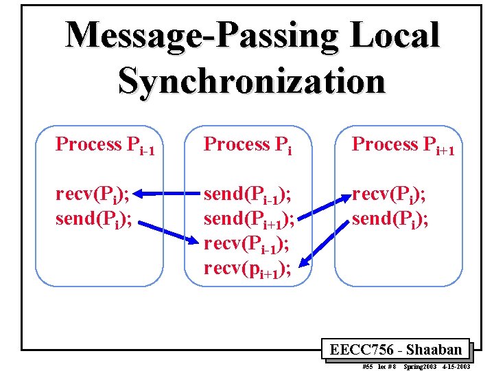
Message-Passing Local Synchronization Process Pi-1 Process Pi+1 recv(Pi); send(Pi); send(Pi-1); send(Pi+1); recv(Pi-1); recv(pi+1); recv(Pi); send(Pi); EECC 756 - Shaaban #55 lec # 8 Spring 2003 4 -15 -2003

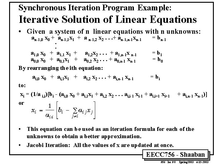
Synchronous Iteration Program Example: Iterative Solution of Linear Equations • Given a system of n linear equations with n unknowns: an-1, 0 x 0 + an-1, 1 x 1 + a n-1, 2 x 2. . . + an-1, n-1 xn-1 = bn-1. . a 1, 0 x 0 + a 1, 1 x 1 + a 1, 2 x 2. . . + a 1, n-1 x n-1 = b 1 a 0, 0 x 0 + a 0, 1 x 1 + a 0, 2 x 2. . . + a 0, n-1 xn-1 = b 0 By rearranging the ith equation: ai, 0 x 0 + ai, 1 x 1 + ai, 2 x 2. . . + ai, n-1 xn-1 = bi to: xi = (1/a i, i)[bi - (ai, 0 x 0 + ai, 1 x 1 + ai, 2 x 2. . . ai, i-1 xi-1 + ai, i+1 xi+1 or + ai, n-1 xn-1)] • This equation can be used as an iteration formula for each of the unknowns to obtain a better approximation. • Jacobi Iteration: All the values of x are updated at once. EECC 756 - Shaaban #56 lec # 8 Spring 2003 4 -15 -2003

Iterative Solution of Linear Equations Jacobi Iteration Sequential Code: • Given the arrays a[][] and b[] holding the constants in the equations, x[] provided to hold the unknowns, and a fixed number of iterations, the code might look like: for (i = 0; i < n; i++) x[i] = b[i]; /* initialize unknowns */ for (iteration = 0; iteration < limit; iteration++) for (i = 0; i < n; i++) sum = 0; for (j = 0; j < n; j++) /* compute summation of a[][]x[] */ if (i != j) { sum = sum + a[i][j] * x[j]; new_x[i] = (b[i] - sum) / a[i][i]; /* Update unknown */ } for (i = 0; i < n; i++) /* update values */ x[i] = new_x[i]; } EECC 756 - Shaaban #57 lec # 8 Spring 2003 4 -15 -2003

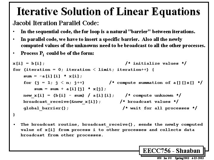
Iterative Solution of Linear Equations Jacobi Iteration Parallel Code: • • • In the sequential code, the for loop is a natural "barrier" between iterations. In parallel code, we have to insert a specific barrier. Also all the newly computed values of the unknowns need to be broadcast to all the other processes. Process Pi could be of the form: x[i] = b[i]; /* initialize values */ for (iteration = 0; iteration < limit; iteration++) { sum = -a[i][i] * x[i]; for (j = 1; j < n; j++) /* compute summation of a[][]x[] */ sum = sum + a[i][j] * x[j]; new_x[i] = (b[i] - sum) / a[i][i]; /* compute unknown */ broadcast_receive(&new_x[i]); /* broadcast values */ global_barrier(); /* wait for all processes */ } • The broadcast routine, broadcast_receive(), sends the newly computed value of x[i] from process i to other processes and collects data broadcast from other processes. EECC 756 - Shaaban #58 lec # 8 Spring 2003 4 -15 -2003

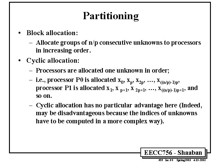
Partitioning • Block allocation: – Allocate groups of n/p consecutive unknowns to processors in increasing order. • Cyclic allocation: – Processors are allocated one unknown in order; – i. e. , processor P 0 is allocated x 0, xp, x 2 p, …, x((n/p)-1)p, processor P 1 is allocated x 1, x p+1, x 2 p+1, …, x((n/p)-1)p+1, and so on. – Cyclic allocation has no particular advantage here (Indeed, may be disadvantageous because the indices of unknowns have to be computed in a more complex way). EECC 756 - Shaaban #59 lec # 8 Spring 2003 4 -15 -2003

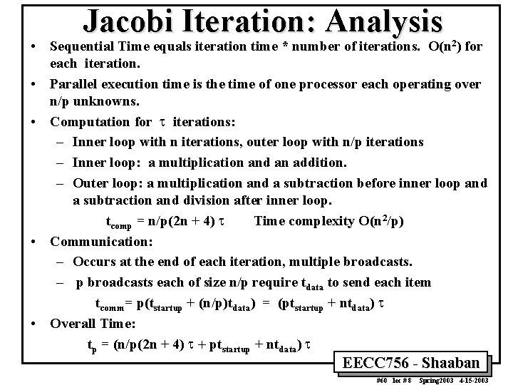
Jacobi Iteration: Analysis • Sequential Time equals iteration time * number of iterations. O(n 2) for each iteration. • Parallel execution time is the time of one processor each operating over n/p unknowns. • Computation for t iterations: – Inner loop with n iterations, outer loop with n/p iterations – Inner loop: a multiplication and an addition. – Outer loop: a multiplication and a subtraction before inner loop and a subtraction and division after inner loop. tcomp = n/p(2 n + 4) t Time complexity O(n 2/p) • Communication: – Occurs at the end of each iteration, multiple broadcasts. – p broadcasts each of size n/p require tdata to send each item tcomm= p(tstartup + (n/p)tdata) = (ptstartup + ntdata) t • Overall Time: tp = (n/p(2 n + 4) t + ptstartup + ntdata) t EECC 756 - Shaaban #60 lec # 8 Spring 2003 4 -15 -2003

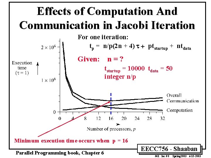
Effects of Computation And Communication in Jacobi Iteration For one iteration: tp = n/p(2 n + 4) t + ptstartup + ntdata Given: n=? tstartup = 10000 tdata = 50 integer n/p Minimum execution time occurs when p = 16 Parallel Programming book, Chapter 6 EECC 756 - Shaaban #61 lec # 8 Spring 2003 4 -15 -2003

Other fully Synchronous Problems: Cellular Automata • The problem space is divided into cells. • Each cell can be in one of a finite number of states. • Cells affected by their neighbors according to certain rules, and all cells are affected simultaneously in a “generation. ” • Rules re-applied in subsequent generations so that cells evolve, or change state, from generation to generation. • Most famous cellular automata is the “Game of Life” devised by John Horton Conway, a Cambridge mathematician. EECC 756 - Shaaban #62 lec # 8 Spring 2003 4 -15 -2003

The Game of Life • Board game - theoretically infinite two-dimensional array of cells. • Each cell can hold one “organism” and has eight neighboring cells, including those diagonally adjacent. Initially, some cells occupied. • The following rules apply: – Every organism with two or three neighboring organisms survives for the next generation. – Every organism with four or more neighbors dies from overpopulation. – Every organism with one neighbor or none dies from isolation. – Each empty cell adjacent to exactly three occupied neighbors will give birth to an organism. • These rules were derived by Conway “after a long period of experimentation. ” EECC 756 - Shaaban #63 lec # 8 Spring 2003 4 -15 -2003

Serious Applications for Cellular Automata • • • Fluid/gas dynamics. The movement of fluids and gases around objects. Diffusion of gases. Biological growth. Airflow across an airplane wing. Erosion/movement of sand at a beach or riverbank. EECC 756 - Shaaban #64 lec # 8 Spring 2003 4 -15 -2003

Dynamic Load Balancing • To achieve best performance of a parallel computing system running a parallel problem, it’s essential to maximize processor utilization by distributing the computation load evenly or balancing the load among the available processors while minimizing overheads. • Optimal static load balancing, mapping or scheduling, is an intractable NP-complete problem, except for specific problems on specific networks. • Hence heuristics are usually used to select processors for processes. • Even the best static mapping may not offer the best execution time due to changing conditions at runtime and the process mapping may need to done dynamically. • The methods used for balancing the computational load dynamically among processors can be broadly classified as: 1. Centralized dynamic load balancing. 2. Decentralized dynamic load balancing. Parallel Programming book, Chapter 7 EECC 756 - Shaaban #65 lec # 8 Spring 2003 4 -15 -2003

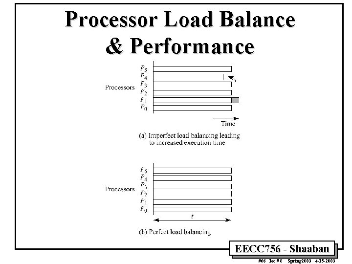
Processor Load Balance & Performance EECC 756 - Shaaban #66 lec # 8 Spring 2003 4 -15 -2003

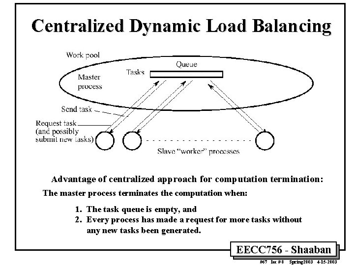
Centralized Dynamic Load Balancing Advantage of centralized approach for computation termination: The master process terminates the computation when: 1. The task queue is empty, and 2. Every process has made a request for more tasks without any new tasks been generated. EECC 756 - Shaaban #67 lec # 8 Spring 2003 4 -15 -2003

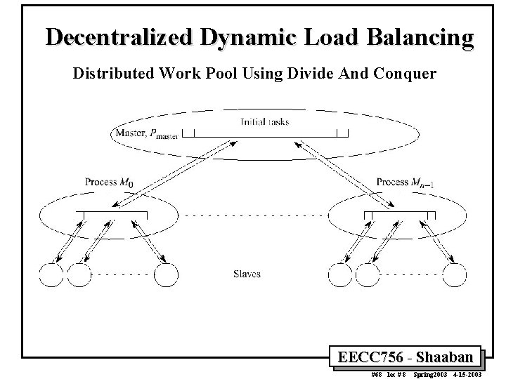
Decentralized Dynamic Load Balancing Distributed Work Pool Using Divide And Conquer EECC 756 - Shaaban #68 lec # 8 Spring 2003 4 -15 -2003

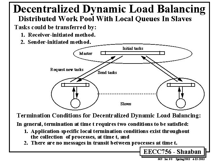
Decentralized Dynamic Load Balancing Distributed Work Pool With Local Queues In Slaves Tasks could be transferred by: 1. Receiver-initiated method. 2. Sender-initiated method. Termination Conditions for Decentralized Dynamic Load Balancing: In general, termination at time t requires two conditions to be satisfied: 1. Application-specific local termination conditions exist throughout the collection of processes, at time t, and 2. There are no messages in transit between processes at time t. EECC 756 - Shaaban #69 lec # 8 Spring 2003 4 -15 -2003

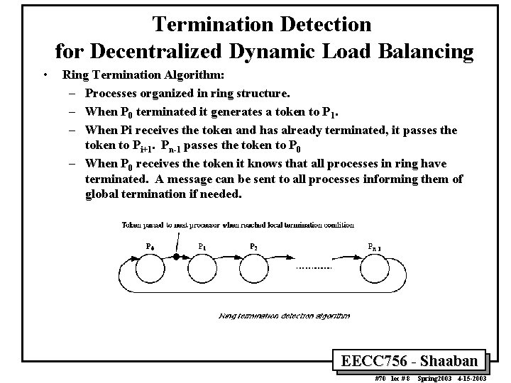
Termination Detection for Decentralized Dynamic Load Balancing • Ring Termination Algorithm: – Processes organized in ring structure. – When P 0 terminated it generates a token to P 1. – When Pi receives the token and has already terminated, it passes the token to Pi+1. Pn-1 passes the token to P 0 – When P 0 receives the token it knows that all processes in ring have terminated. A message can be sent to all processes informing them of global termination if needed. EECC 756 - Shaaban #70 lec # 8 Spring 2003 4 -15 -2003

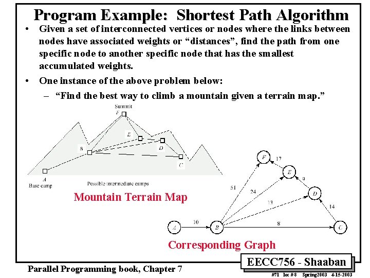
Program Example: Shortest Path Algorithm • Given a set of interconnected vertices or nodes where the links between nodes have associated weights or “distances”, find the path from one specific node to another specific node that has the smallest accumulated weights. • One instance of the above problem below: – “Find the best way to climb a mountain given a terrain map. ” Mountain Terrain Map Corresponding Graph EECC 756 - Shaaban Parallel Programming book, Chapter 7 #71 lec # 8 Spring 2003 4 -15 -2003

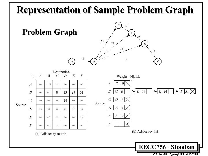
Representation of Sample Problem Graph EECC 756 - Shaaban #72 lec # 8 Spring 2003 4 -15 -2003

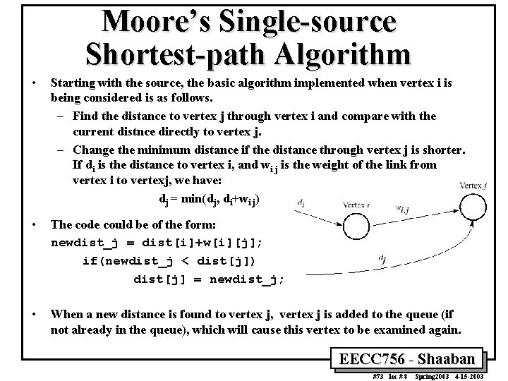
Moore’s Single-source Shortest-path Algorithm • Starting with the source, the basic algorithm implemented when vertex i is being considered is as follows. – Find the distance to vertex j through vertex i and compare with the current distnce directly to vertex j. – Change the minimum distance if the distance through vertex j is shorter. If di is the distance to vertex i, and wi j is the weight of the link from vertex i to vertexj, we have: dj = min(dj, di+wi j) • The code could be of the form: newdist_j = dist[i]+w[i][j]; if(newdist_j < dist[j]) dist[j] = newdist_j; • When a new distance is found to vertex j, vertex j is added to the queue (if not already in the queue), which will cause this vertex to be examined again. EECC 756 - Shaaban #73 lec # 8 Spring 2003 4 -15 -2003

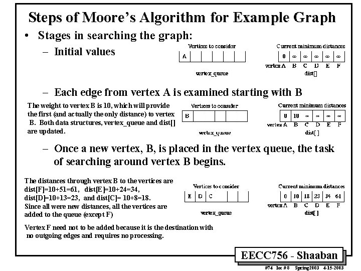
Steps of Moore’s Algorithm for Example Graph • Stages in searching the graph: – Initial values – Each edge from vertex A is examined starting with B The weight to vertex B is 10, which will provide the first (and actually the only distance) to vertex B. Both data structures, vertex_queue and dist[] are updated. – Once a new vertex, B, is placed in the vertex queue, the task of searching around vertex B begins. The distances through vertex B to the vertices are dist[F]=10+51=61, dist[E]=10+24=34, dist[D]=10+13=23, and dist[C]= 10+8=18. Since all were new distances, all the vertices are added to the queue (except F) Vertex F need not to be added because it is the destination with no outgoing edges and requires no processing. EECC 756 - Shaaban #74 lec # 8 Spring 2003 4 -15 -2003

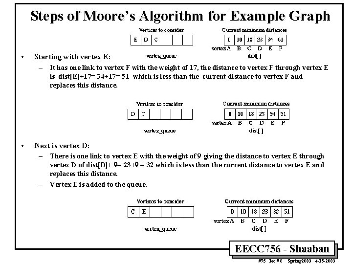
Steps of Moore’s Algorithm for Example Graph • Starting with vertex E: – It has one link to vertex F with the weight of 17, the distance to vertex F through vertex E is dist[E]+17= 34+17= 51 which is less than the current distance to vertex F and replaces this distance. • Next is vertex D: – There is one link to vertex E with the weight of 9 giving the distance to vertex E through vertex D of dist[D]+ 9= 23+9 = 32 which is less than the current distance to vertex E and replaces this distance. – Vertex E is added to the queue. EECC 756 - Shaaban #75 lec # 8 Spring 2003 4 -15 -2003

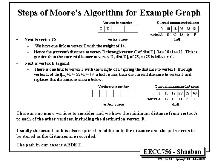
Steps of Moore’s Algorithm for Example Graph • Next is vertex C: – We have one link to vertex D with the weight of 14. – Hence the (current) distance to vertex D through vertex C of dist[C]+14= 18+14=32. This is greater than the current distance to vertex D, dist[D], of 23, so 23 is left stored. • Next is vertex E (again): – There is one link to vertex F with the weight of 17 giving the distance to vertex F through vertex E of dist[E]+17= 32+17=49 which is less than the current distance to vertex F and replaces this distance, as shown below: There are no more vertices to consider and we have the minimum distance from vertex A to each of the other vertices, including the destination vertex, F. Usually the actual path is also required in addition to the distance and the path needs to be stored as the distances are recorded. The path in our case is ABDE F. EECC 756 - Shaaban #76 lec # 8 Spring 2003 4 -15 -2003

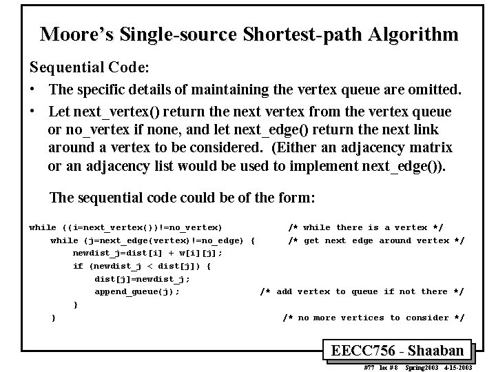
Moore’s Single-source Shortest-path Algorithm Sequential Code: • The specific details of maintaining the vertex queue are omitted. • Let next_vertex() return the next vertex from the vertex queue or no_vertex if none, and let next_edge() return the next link around a vertex to be considered. (Either an adjacency matrix or an adjacency list would be used to implement next_edge()). The sequential code could be of the form: while ((i=next_vertex())!=no_vertex) /* while there is a vertex */ while (j=next_edge(vertex)!=no_edge) { /* get next edge around vertex */ newdist_j=dist[i] + w[i][j]; if (newdist_j < dist[j]) { dist[j]=newdist_j; append_gueue(j); /* add vertex to queue if not there */ } } /* no more vertices to consider */ EECC 756 - Shaaban #77 lec # 8 Spring 2003 4 -15 -2003

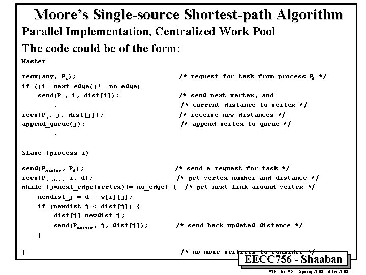
Moore’s Single-source Shortest-path Algorithm Parallel Implementation, Centralized Work Pool The code could be of the form: Master recv(any, Pi); if ((i= next_edge()!= no_edge) send(Pi, i, dist[i]); . recv(Pj, j, dist[j]); append_gueue(j); . /* request for task from process Pi */ /* /* send next vertex, and current distance to vertex */ receive new distances */ append vertex to queue */ Slave (process i) send(Pmaster, Pi); /* send a request for task */ recv(Pmaster, i, d); /* get vertex number and distance */ while (j=next_edge(vertex)!= no_edge) { /* get next link around vertex */ newdist_j = d + w[i][j]; if (newdist_j < dist[j]) { dist[j]=newdist_j; send(Pmaster, j, dist[j]); /* send back updated distance */ } } /* no more vertices to consider */ EECC 756 - Shaaban #78 lec # 8 Spring 2003 4 -15 -2003

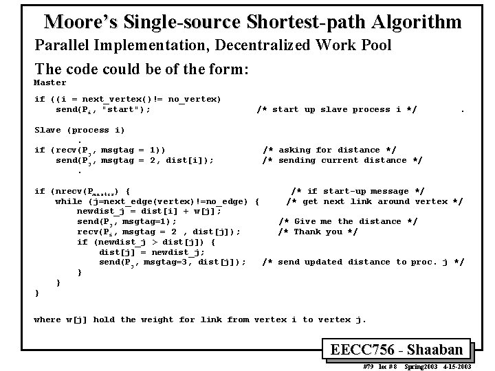
Moore’s Single-source Shortest-path Algorithm Parallel Implementation, Decentralized Work Pool The code could be of the form: Master if ((i = next_vertex()!= no_vertex) send(Pi, "start"); Slave (process i). if (recv(Pj, msgtag = 1)) send(Pj, msgtag = 2, dist[i]); . /* start up slave process i */ . /* asking for distance */ /* sending current distance */ if (nrecv(Pmaster) { /* if start-up message */ while (j=next_edge(vertex)!=no_edge) { /* get next link around vertex */ newdist_j = dist[i] + w[j]; send(Pj, msgtag=1); /* Give me the distance */ recv(Pi, msgtag = 2 , dist[j]); /* Thank you */ if (newdist_j > dist[j]) { dist[j] = newdist_j; send(Pj, msgtag=3, dist[j]); /* send updated distance to proc. j */ } } } where w[j] hold the weight for link from vertex i to vertex j. EECC 756 - Shaaban #79 lec # 8 Spring 2003 4 -15 -2003

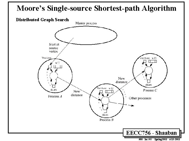
Moore’s Single-source Shortest-path Algorithm Distributed Graph Search EECC 756 - Shaaban #80 lec # 8 Spring 2003 4 -15 -2003