Basic Numerical Procedure 1 Content 1 Binomial Trees

Basic Numerical Procedure 1

Content 1 Binomial Trees 2 Using the binomial tree for options on indices, currencies, and futures contracts 3 Binomial model for a dividend-paying stock 4 Alternative procedures for constructing trees 5 Time-dependent parameters 6 Monte Carlo simulation 7 Variance reduction procedures 8 Finite difference methods 2

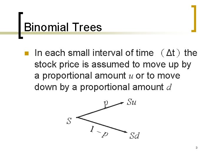
Binomial Trees n In each small interval of time （Δt）the stock price is assumed to move up by a proportional amount u or to move down by a proportional amount d S p Su 1–p Sd 3

Risk-Neutral Valuation 1. Assume that the expected return from all traded assets is the risk-free interest rate. 2. Value payoffs from the derivative by calculating their expected values and discounting at the risk-free interest rate. 4

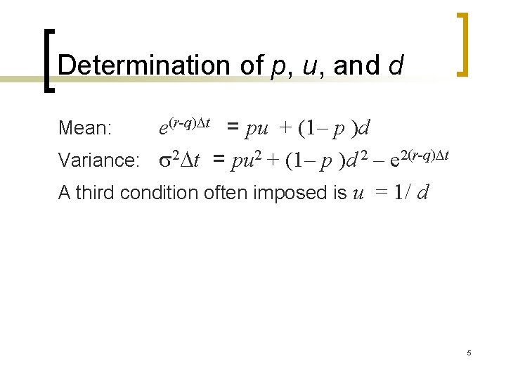
Determination of p, u, and d e(r-q)Dt = pu + (1– p )d Variance: s 2 Dt = pu 2 + (1– p )d 2 – e 2(r-q)Dt A third condition often imposed is u = 1/ d Mean: 5

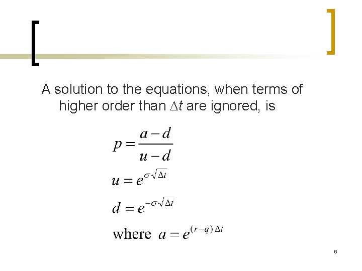
A solution to the equations, when terms of higher order than Dt are ignored, is 6

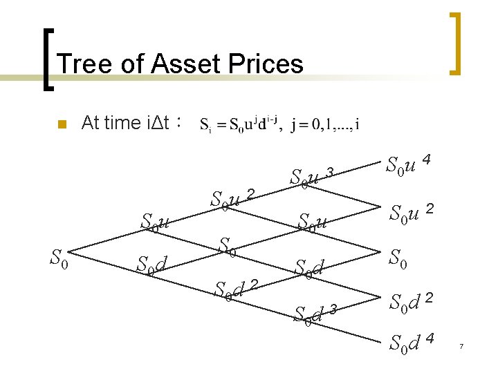
Tree of Asset Prices n At time iΔt： S 0 u S 0 d S 0 u 2 S 0 d 2 S 0 u 3 S 0 u 4 S 0 u 2 S 0 d 3 S 0 d 2 S 0 d 4 7

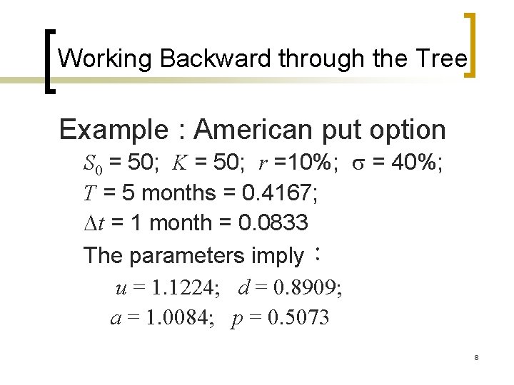
Working Backward through the Tree Example : American put option S 0 = 50; K = 50; r =10%; s = 40%; T = 5 months = 0. 4167; Dt = 1 month = 0. 0833 The parameters imply： u = 1. 1224; d = 0. 8909; a = 1. 0084; p = 0. 5073 8

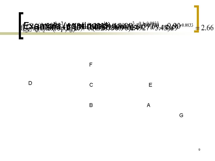
Example (continued) F D C B E A G 9

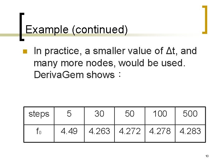
Example (continued) n In practice, a smaller value of Δt, and many more nodes, would be used. Deriva. Gem shows： steps 5 f 0 4. 49 30 50 100 500 4. 263 4. 272 4. 278 4. 283 10

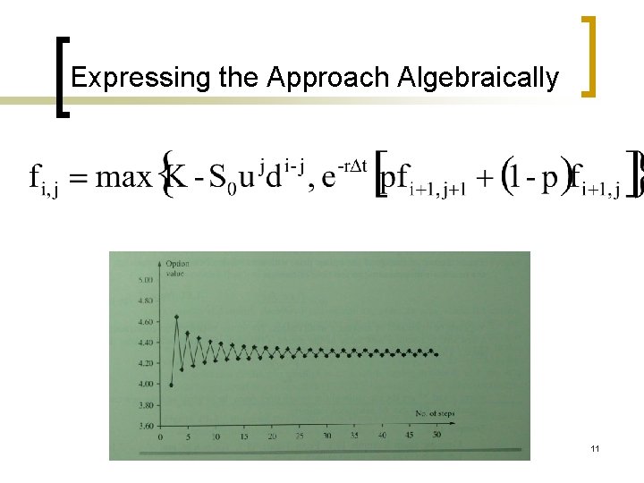
Expressing the Approach Algebraically 11

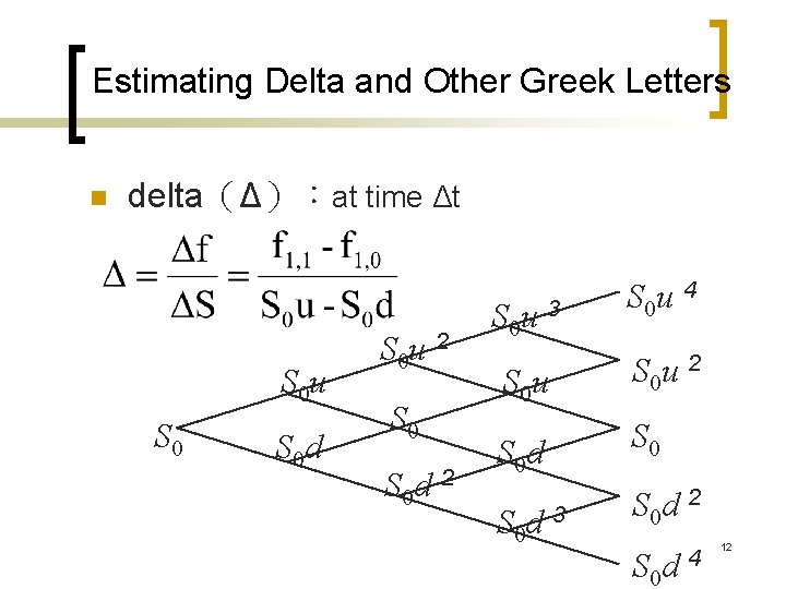
Estimating Delta and Other Greek Letters n delta（Δ）：at time Δt S 0 u S 0 d S 0 u 2 S 0 d 2 S 0 u 3 S 0 u 4 S 0 u 2 S 0 d 3 S 0 d 2 S 0 d 4 12

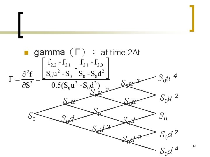
n gamma（Γ）： at time 2Δt S 0 u S 0 d S 0 u 2 S 0 d 2 S 0 u 3 S 0 u 4 S 0 u 2 S 0 d 3 S 0 d 2 S 0 d 4 13

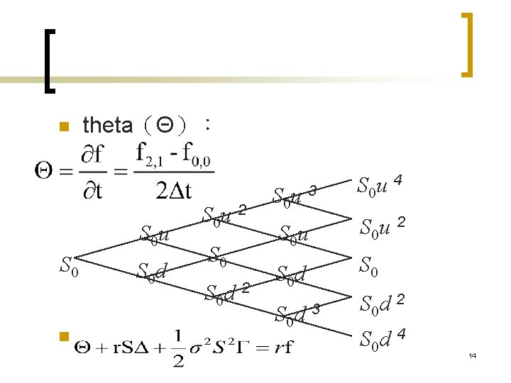
n theta（Θ）： S 0 u S 0 n S 0 d S 0 u 2 S 0 d 2 S 0 u 3 S 0 u 4 S 0 u 2 S 0 d 3 S 0 d 2 S 0 d 4 14

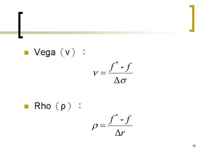
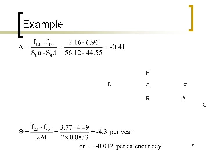
Example F D C E B A G 16

Using the binomial tree for options on indices, currencies, and futures contracts As with Black-Scholes： ¡ For options on stock indices, q equals the dividend yield on the index ¡ For options on a foreign currency, q equals the foreign risk-free rate ¡ For options on futures contracts： q = r 17

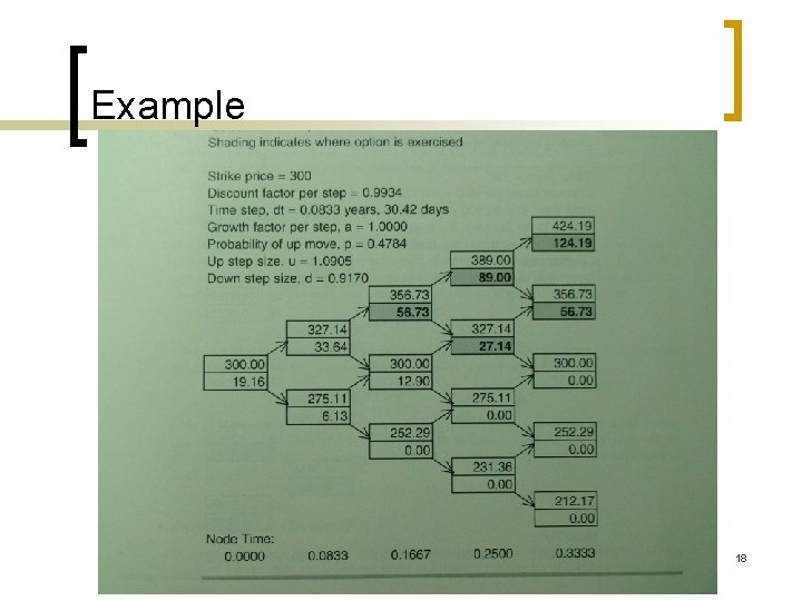
Example 18

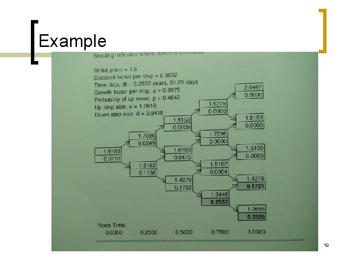
Example 19

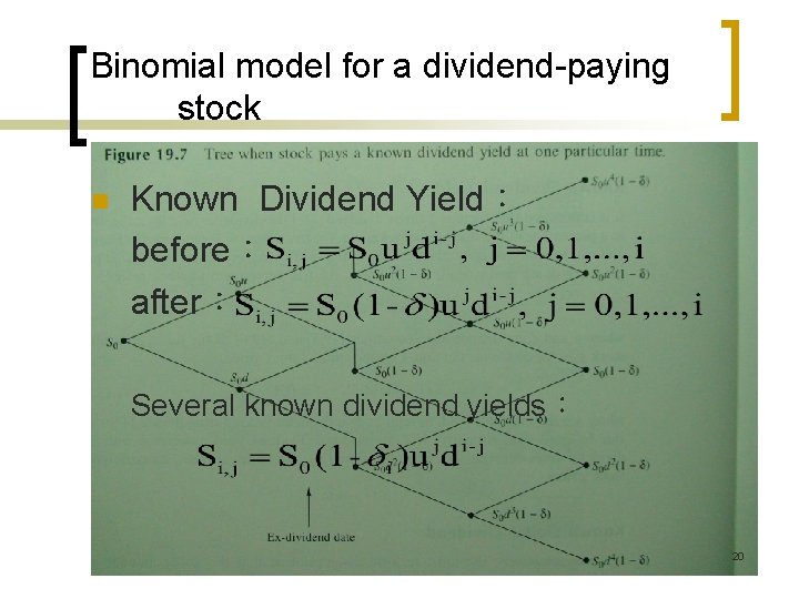
Binomial model for a dividend-paying stock n Known Dividend Yield： before： after： Several known dividend yields： 20

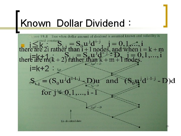
Known Dollar Dividend： n i≦k： i=k+1： i=k+2： 21

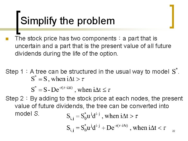
Simplify the problem n The stock price has two components：a part that is uncertain and a part that is the present value of all future dividends during the life of the option. Step 1：A tree can be structured in the usual way to model . Step 2：By adding to the stock price at each nodes, the present value of future dividends, the tree can be converted into model S. 22

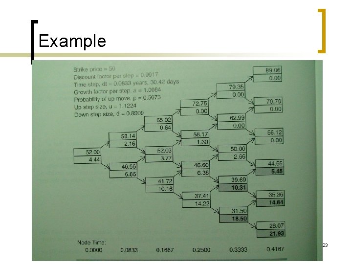
Example 23

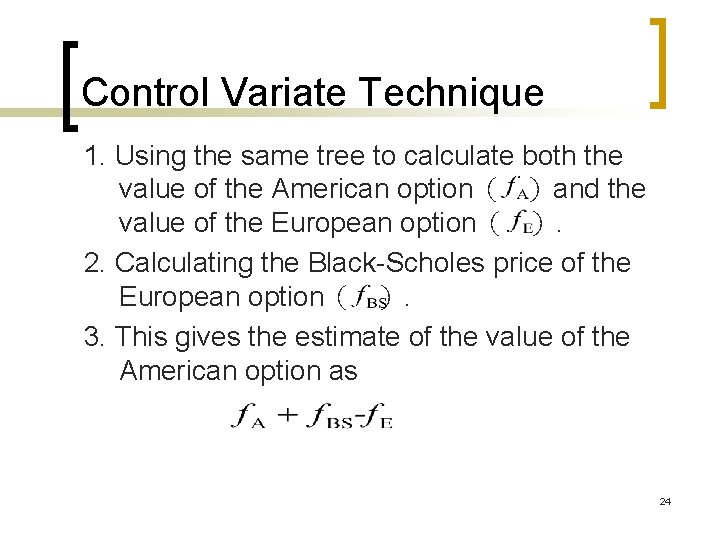
Control Variate Technique 1. Using the same tree to calculate both the value of the American option（ ）and the value of the European option（ ）. 2. Calculating the Black-Scholes price of the European option（ ）. 3. This gives the estimate of the value of the American option as 24

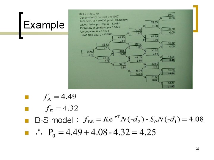
Example n n B-S model： ∴ 25

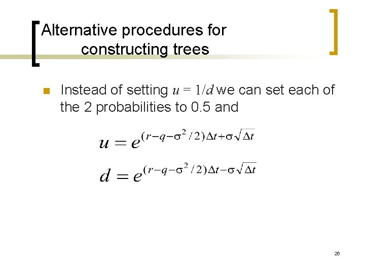
Alternative procedures for constructing trees n Instead of setting u = 1/d we can set each of the 2 probabilities to 0. 5 and 26

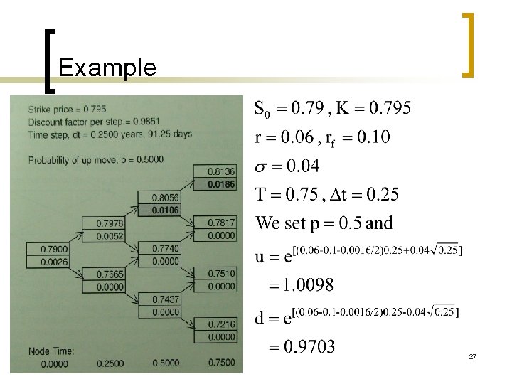
Example 27

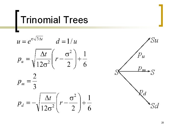
Trinomial Trees Su pu S pm S pd Sd 28

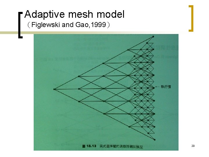
Adaptive mesh model （Figlewski and Gao, 1999） 29

Time-dependent parameters 30

Monte Carlo simulation n 1. 2. 3. 4. 5. When used to value an option, Monte Carlo simulation uses the risk-neutral valuation result. It involves the following steps: Simulate a random path for S in a risk neutral world. Calculate the payoff from the derivative. Repeat steps 1 and 2 to get many sample values of the payoff from the derivative in a risk neutral world. Calculate the mean of the sample payoffs to get an estimate of the expected payoff. Discount this expected payoff at risk-free rate to get an estimate of the value of the derivative. 31

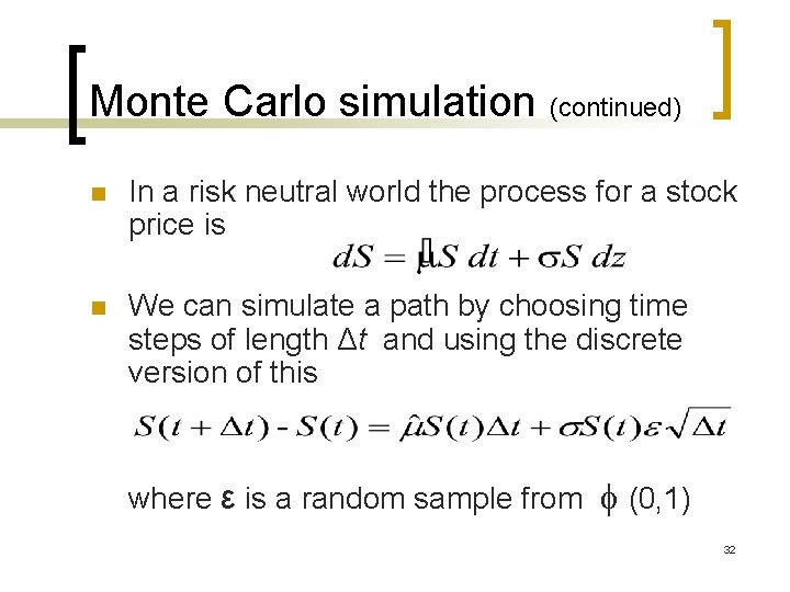
Monte Carlo simulation (continued) n In a risk neutral world the process for a stock price is n We can simulate a path by choosing time steps of length Δt and using the discrete version of this where ε is a random sample from f (0, 1) 32

Monte Carlo simulation (continued) 33

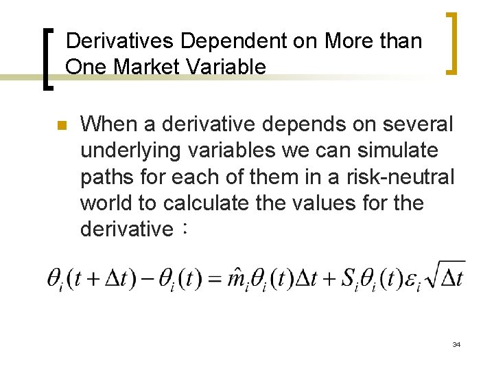
Derivatives Dependent on More than One Market Variable n When a derivative depends on several underlying variables we can simulate paths for each of them in a risk-neutral world to calculate the values for the derivative： 34

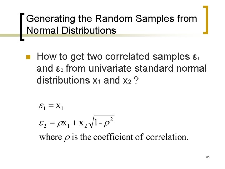
Generating the Random Samples from Normal Distributions n How to get two correlated samples ε 1 and ε 2 from univariate standard normal distributions x 1 and x 2？ 35

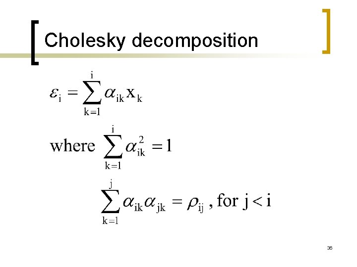
Cholesky decomposition 36

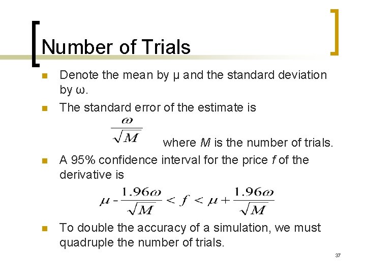
Number of Trials n n Denote the mean by μ and the standard deviation by ω. The standard error of the estimate is where M is the number of trials. A 95% confidence interval for the price f of the derivative is To double the accuracy of a simulation, we must quadruple the number of trials. 37

Applications n Advantage： 1. It tends to be numerically more efficient （ increases linearly）than other procedures（ increases exponentially）when there are more stochastic variables. 2. It can provide a standard error for the estimates. 3. It is an approach that can accommodate complex payoffs and complex stocastic processes. 38

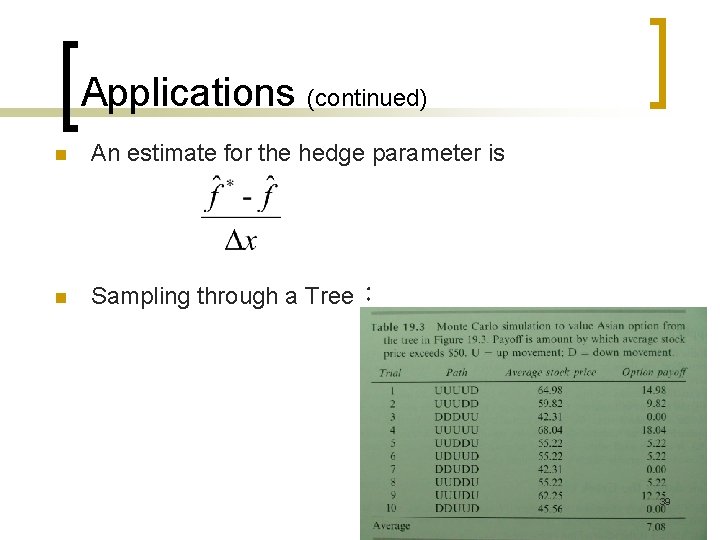
Applications (continued) n An estimate for the hedge parameter is n Sampling through a Tree： 39

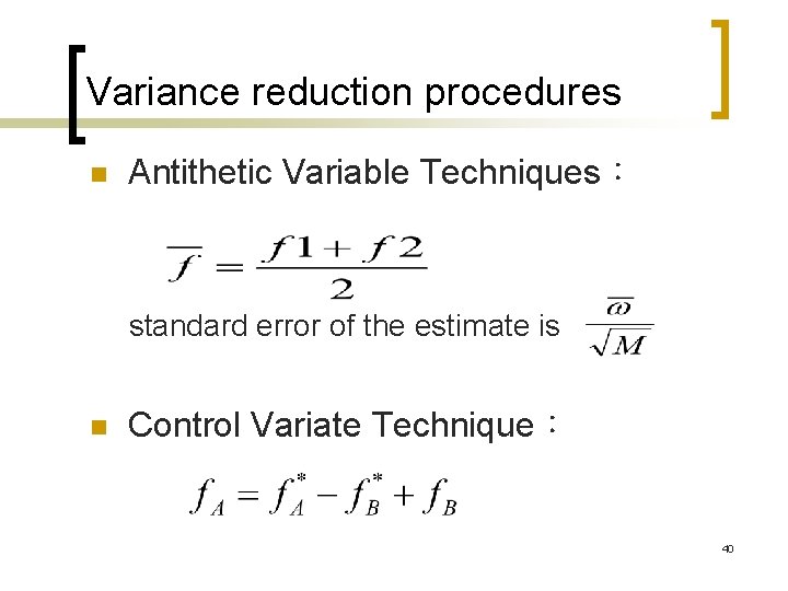
Variance reduction procedures n Antithetic Variable Techniques： standard error of the estimate is n Control Variate Technique： 40

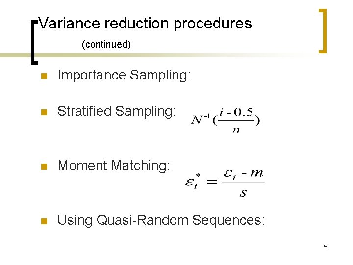
Variance reduction procedures (continued) n Importance Sampling: n Stratified Sampling: n Moment Matching: n Using Quasi-Random Sequences: 41

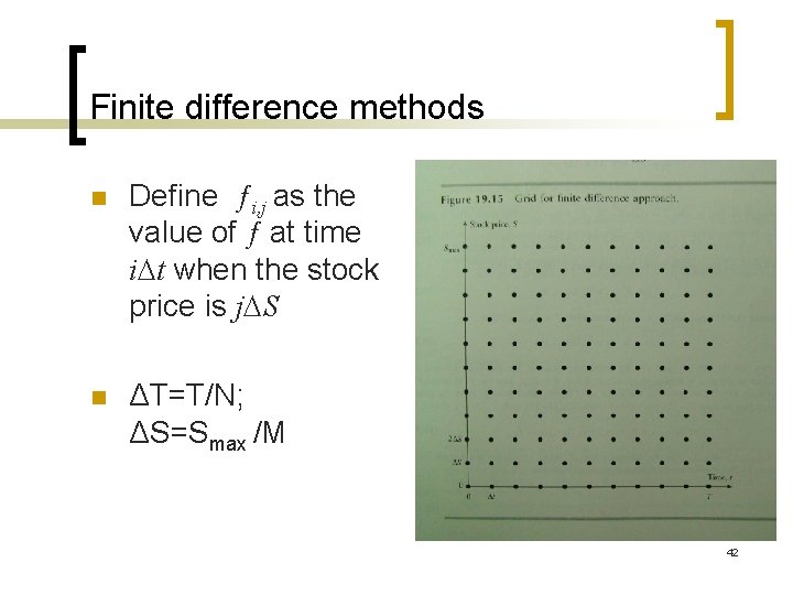
Finite difference methods n Define ƒi, j as the value of ƒ at time i. Dt when the stock price is j. DS n ΔT=T/N; ΔS=Smax /M 42

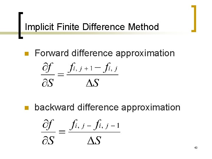
Implicit Finite Difference Method n Forward difference approximation n backward difference approximation 43

Implicit Finite Difference Methods (continued) 44

Implicit Finite Difference Methods (continued) 45

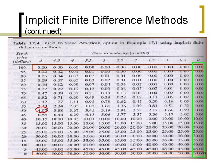
Implicit Finite Difference Methods (continued) 46

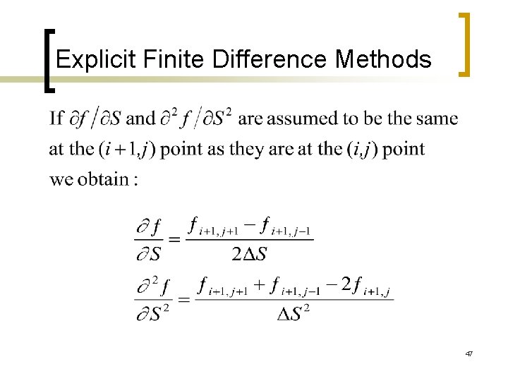
Explicit Finite Difference Methods 47

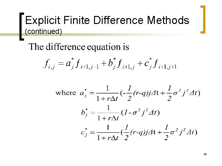
Explicit Finite Difference Methods (continued) 48

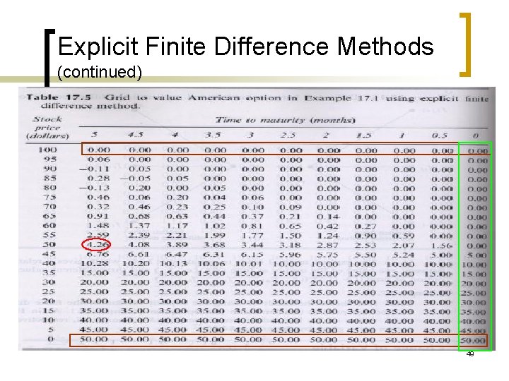
Explicit Finite Difference Methods (continued) 49

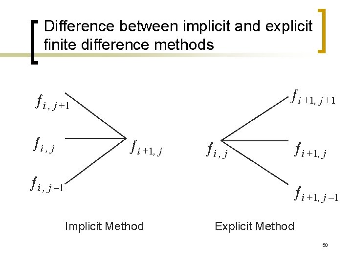
Difference between implicit and explicit finite difference methods ƒi +1, j +1 ƒi , j ƒi +1, j ƒi , j – 1 ƒi , j ƒi +1, j – 1 Implicit Method Explicit Method 50

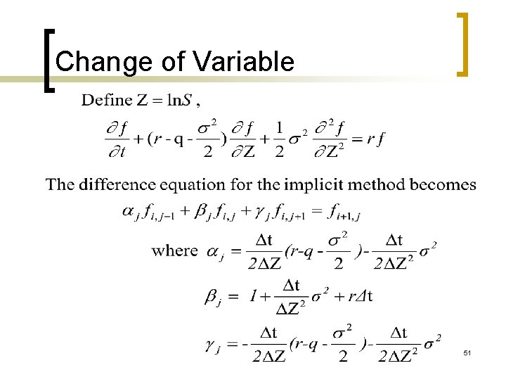
Change of Variable 51

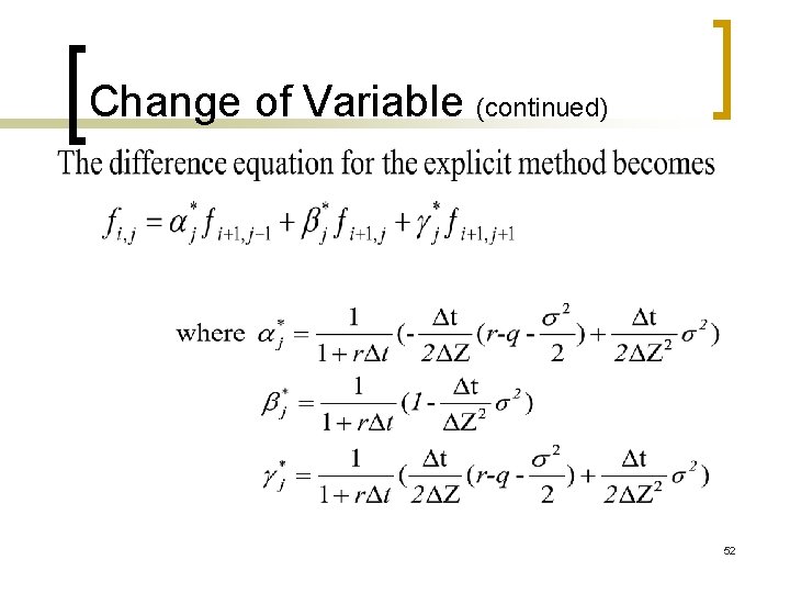
Change of Variable (continued) 52

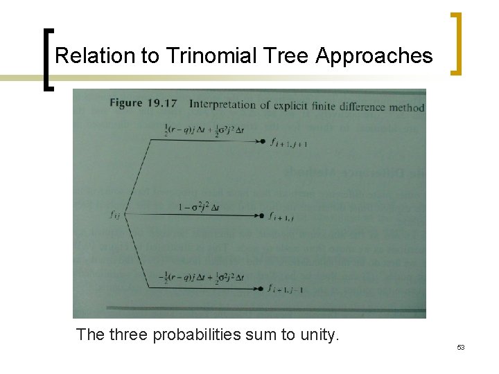
Relation to Trinomial Tree Approaches The three probabilities sum to unity. 53

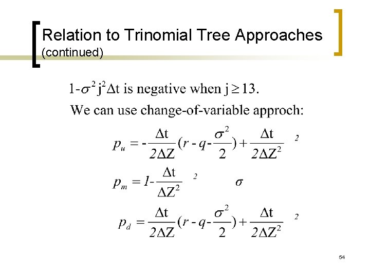
Relation to Trinomial Tree Approaches (continued) 54

Other Finite Difference Methods n Hopscotch method n Crank-Nicolson scheme n Quadratic approximation 55

Summary n n We have three different numerical procedures for valuing derivatives when no analytic solution: trees, Monte Carlo simulation, and finite difference methods. Trees: derivative price are calculated by starting at the end of the tree and working backwards. Monte Carlo simulation: works forward from the beginning, and becomes relatively more efficient as the number of underlying variables increases. Finite difference method: similar to tree approaches. The implicit finite difference method is more complicated but has the advantage that does not have to take any special precautions to ensure convergence. 56