Basic GIS Functions and Spatial Stats in Packages

Basic GIS Functions and Spatial Stats in

Packages Needed Today • Require command will install packages and any packages it depends on • What we need require(sp) require(rgdal) require(rgeos) require(raster) require(spatstat) require(spdep) require(RANN) require(gstat) require(adehabitat. HR) require(ROCR) require(SDMTools)

Getting Started with Vector Data Packages: >library (sp) • Provides classes and methods for spatial data >library (rgdal) • Provides bindings to Frank Warmerdam's Geospatial Data Abstraction Library >library (rgeos) • Provides geostatistical functions such as regression and basic shapefile operations • • • Other Useful Vector Data Packages > library(maptools) > library(shapefiles) > library(spatstat) > library(splancs)

Getting Started with Vector Data • Loading Sample Data • OGR -> Open. GIS Simple Features Reference Implementation • Dsn -> “data set name” • Cactus Point file >cactus<- read. OGR(dsn=getwd(), layer="Cactus") • Streams Line File >strm<- read. OGR(dsn=getwd(), layer="NHD_Streams") • Study Area Polygon >stdy<- read. OGR(dsn=getwd(), layer="Study. Area")

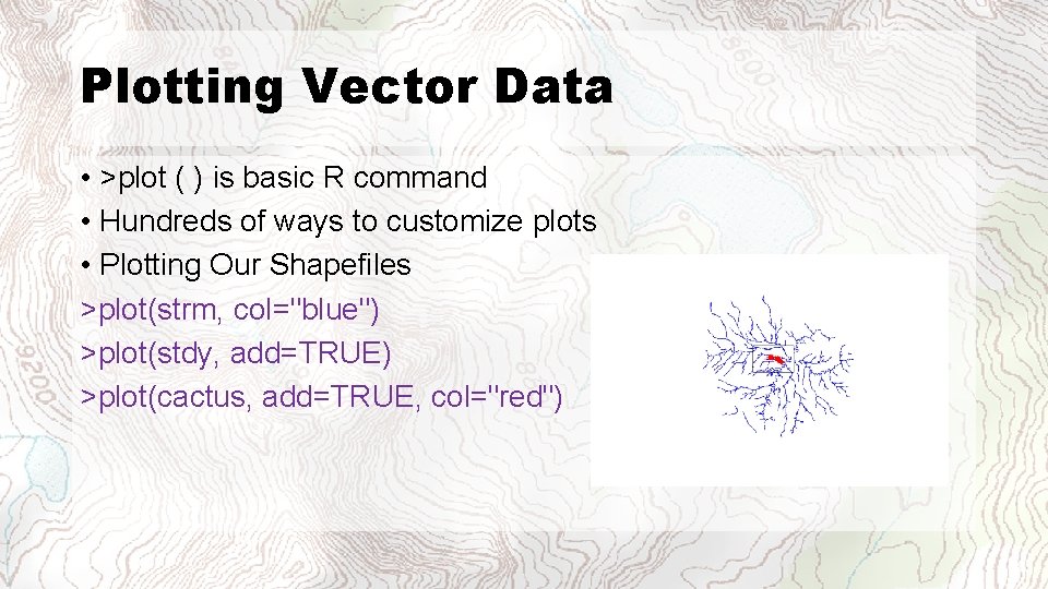
Plotting Vector Data • >plot ( ) is basic R command • Hundreds of ways to customize plots • Plotting Our Shapefiles >plot(strm, col="blue") >plot(stdy, add=TRUE) >plot(cactus, add=TRUE, col="red")

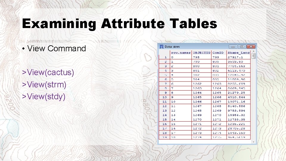
Examining Attribute Tables • View Command >View(cactus) >View(strm) >View(stdy)

Looking Under the Hood >str(stdy) • 'slots' (data, polygons(or lines or coords), plot. Order, bbox, proj 4 string) • These mimic the file structure of a shapefile • @data = the *. dbf = the attribute table • @polygons/lines/coords = *. shp = the geometries that define the spatial components • @bbox = the extent of the object(s) in rectangular form • @proj 4 string = *. prj = the projection file describing how to draw the coordinates in space

Examining Attribute Tables • In this example we are retrieving the 5 th line from the Stream Shapefile Attribute Table >strm[5, ] • We can plot this as well >plot(strm[5, ]) • This logic works for retrieving only the attribute table information. • Thus @data is simply a data. frame() associated with spatial features >strm@data[5, ]

Basic Spatial Analysis – Intersecting Geometries • Intersect geometries • Rgeos • Intersect the study area streams cropped by the boundary >istrm<- g. Intersection(strm, stdy, byid=TRUE) • This is a set of streams that do not have attributes associated with them • The byid=TRUE maintains each stream as unique feature instead of dissolving. • Matching the attributes can be troublesome

Basic Spatial Analysis – Intersecting Geometries • The Fix • Strip off the 0 >row. names(istrm)<- as. character(sapply(row. names(istrm), FUN=function(x){strsplit(x, " ")[[1]][1]})) • Match the attributes from the full set of streams with the intersected streams >istrm<- Spatial. Lines. Data. Frame(istrm, data=strm@data[which(!is. na(match(row. names(strm), row. names(istrm)))), ]) >View(istrm)

Basic Spatial Analysis – Intersecting Geometries • Plot our new dataset >plot(istrm, col="blue") >plot(stdy, add=TRUE) >plot(cactus, add=TRUE, col="red")

Basic Spatial Analysis – Merge • Now that we have practiced adding attributes back to an 'rgeos' derived vector layer • We need to actually dissolve these streams into one feature for easier processing in future steps >istrm<- g. Line. Merge(istrm) • The cool thing is that the clipped streams are in-memory. So, if you want to perform other stuff on the results, you can without having to store temporary shapefiles, etc. . .

Basic Spatial Analysis – Buffering • Buffering points >pbuff<- g. Buffer(cactus, byid=TRUE, width=1000) • Now we have to add the attributes back to the buffers. This is a 1 to 1, so the attributes don't need manipulation >pbuff<- Spatial. Polygons. Data. Frame(pbuff, cactus@data, match. ID=TRUE) >plot(pbuff, add=TRUE)

Basic Spatial Analysis – Clipping • Clip the areas from the study area that fall within the point buffer • Rgeos • Dissolve the buffered points first >pdis<- g. Unary. Union(pbuff) • Get the geometric difference >pdiff<- g. Difference(stdy, pdis) #; rgeos >plot(pdiff, col="red")

Basic Spatial Analysis – Building Polygons • We are going to expand the study extent to match a buffer size and reduce the edge effect of zonal stats (for later) • Let's build a polygon from scratch. To create a true polygon feature class, we need to deal with the spatial hierarchy >xs<- c((bbox(stdy)[1, 1]-1000), (bbox(stdy)[1, 2]+1000), (bbox(stdy)[1, 1]-1000), (bbox(stdy)[1, 1]1000)) >ys<- c((bbox(stdy)[2, 1]-1000), (bbox(stdy)[2, 2]+1000), (bbox(stdy)[2, 1]1000))

Basic Spatial Analysis – Building Polygons • Create a single polygon >rstdy<- Polygon(matrix(c(xs, ys), ncol=2)) • Create a list of polygons (yes we only have one, but. . . ) >rstdy<- Polygons(list(rstdy), ID="1") • Now make it spatially aware >rstdy<- Spatial. Polygons(list(rstdy), >proj 4 string=CRS(proj 4 string(stdy)))

Basic Spatial Analysis – Building Points • Create random points and append them to our cactus points. Use the reduced extent >rp<- spsample(stdy, n=length(cactus[, 1]), type="random") • Add attribute table to random points >rp<- Spatial. Points. Data. Frame(rp, data=data. frame(Point. ID=1: nrow(cactus), Present=0)) • Append the random points to the cactus points >cactus<- rbind(cactus, rp)

Basic Spatial Analysis – Building Points • View the attributes >View(cactus@data) • Map the points >plot(stdy) >plot(cactus, col=ifelse(cactus@data$Present==1, "black", "red"), add=TRUE)

Basic Spatial Analysis – Find distance between 2 geometries • VECTOR method • Transpose the returned matrix >pdist<- t(g. Distance(cactus, istrm, byid=TRUE)) • Get the average distance to the streams >mean(pdist) • Get the minimum distance to the streams >min(pdist) • Add the results to the in-memory point shapefile >cactus@data<- data. frame(cactus@data, Strm. Dist= pdist[match(rownames(cactus@data), rownames(pdist)), ]) >View(cactus@data)

Basic Spatial Analysis – Raster Data • First we need to read in the raster data >dem<- raster("DEM_30 m. img") >plot(dem) >plot(stdy, add=TRUE, col="red")

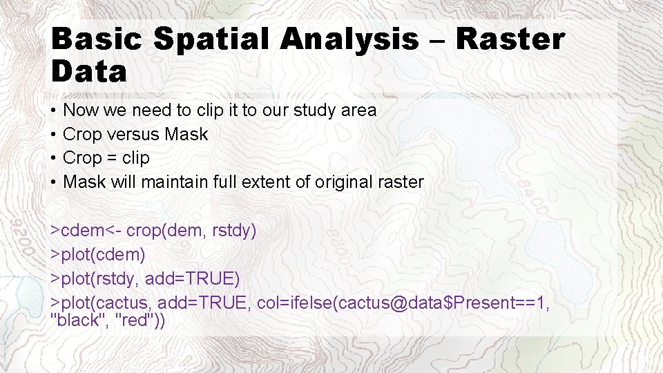
Basic Spatial Analysis – Raster Data • • Now we need to clip it to our study area Crop versus Mask Crop = clip Mask will maintain full extent of original raster >cdem<- crop(dem, rstdy) >plot(cdem) >plot(rstdy, add=TRUE) >plot(cactus, add=TRUE, col=ifelse(cactus@data$Present==1, "black", "red"))

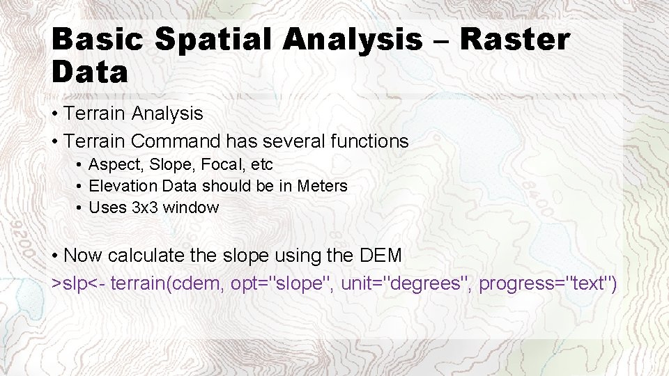
Basic Spatial Analysis – Raster Data • Terrain Analysis • Terrain Command has several functions • Aspect, Slope, Focal, etc • Elevation Data should be in Meters • Uses 3 x 3 window • Now calculate the slope using the DEM >slp<- terrain(cdem, opt="slope", unit="degrees", progress="text")

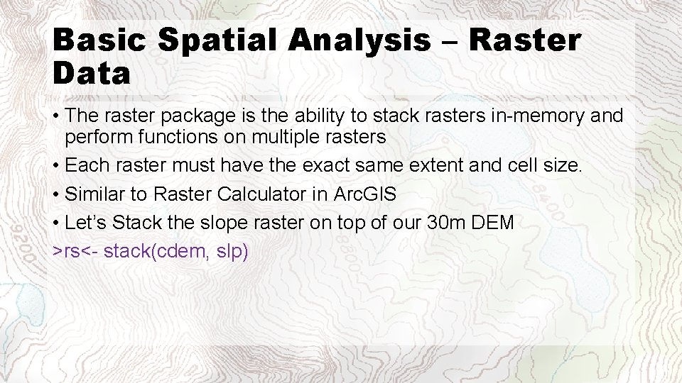
Basic Spatial Analysis – Raster Data • The raster package is the ability to stack rasters in-memory and perform functions on multiple rasters • Each raster must have the exact same extent and cell size. • Similar to Raster Calculator in Arc. GIS • Let’s Stack the slope raster on top of our 30 m DEM >rs<- stack(cdem, slp)

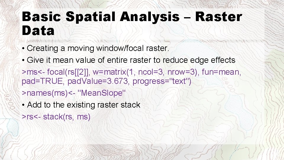
Basic Spatial Analysis – Raster Data • Creating a moving window/focal raster. • Give it mean value of entire raster to reduce edge effects >ms<- focal(rs[[2]], w=matrix(1, ncol=3, nrow=3), fun=mean, pad=TRUE, pad. Value=3. 673, progress="text") >names(ms)<- "Mean. Slope" • Add to the existing raster stack >rs<- stack(rs, ms)

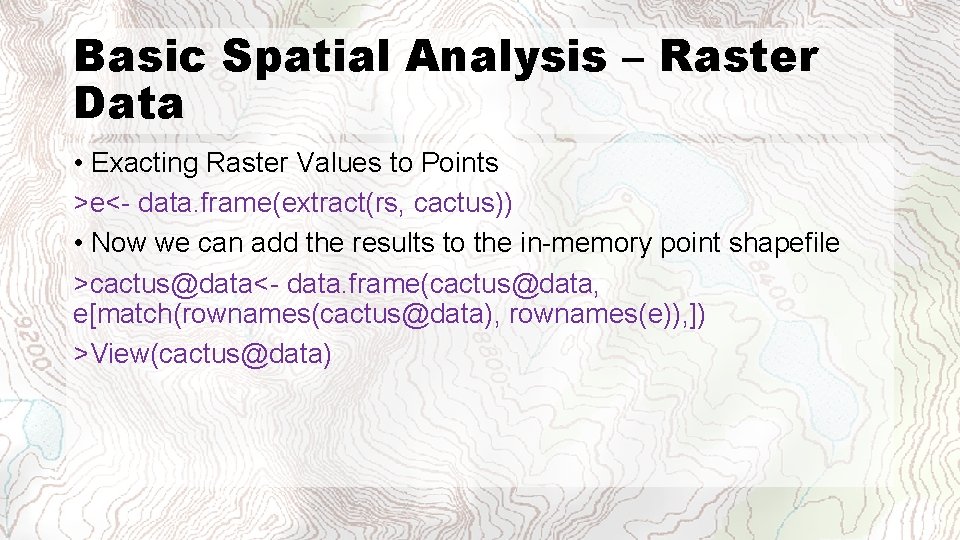
Basic Spatial Analysis – Raster Data • Exacting Raster Values to Points >e<- data. frame(extract(rs, cactus)) • Now we can add the results to the in-memory point shapefile >cactus@data<- data. frame(cactus@data, e[match(rownames(cactus@data), rownames(e)), ]) >View(cactus@data)

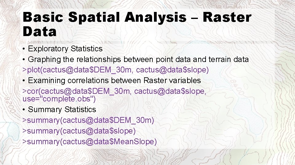
Basic Spatial Analysis – Raster Data • Exploratory Statistics • Graphing the relationships between point data and terrain data >plot(cactus@data$DEM_30 m, cactus@data$slope) • Examining correlations between Raster variables >cor(cactus@data$DEM_30 m, cactus@data$slope, use="complete. obs") • Summary Statistics >summary(cactus@data$DEM_30 m) >summary(cactus@data$slope) >summary(cactus@data$Mean. Slope)

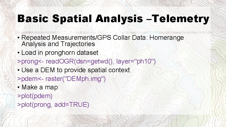
Basic Spatial Analysis –Telemetry • Repeated Measurements/GPS Collar Data: Homerange Analysis and Trajectories • Load in pronghorn dataset >prong<- read. OGR(dsn=getwd(), layer="ph 10") • Use a DEM to provide spatial context >pdem<- raster("DEMph. img") • Make a map >plot(pdem) >plot(prong, add=TRUE)

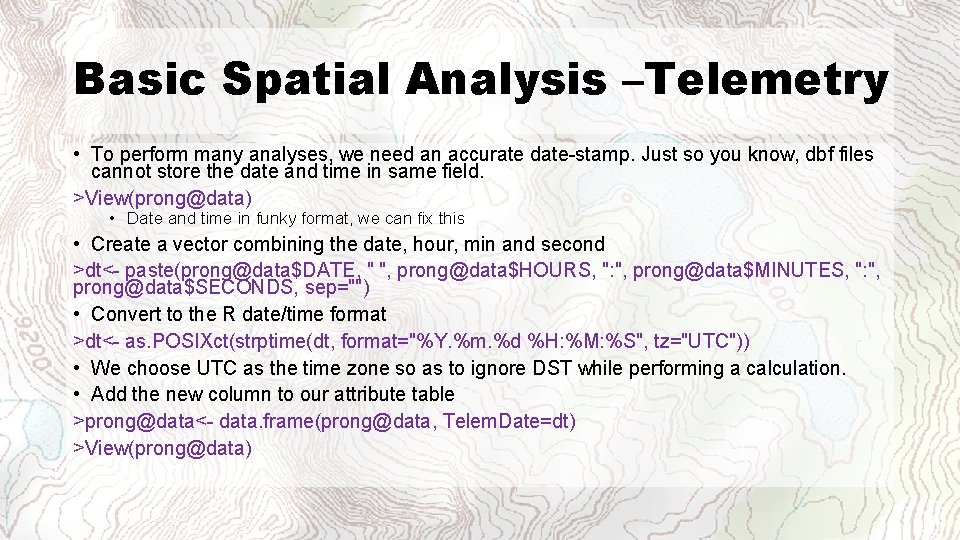
Basic Spatial Analysis –Telemetry • To perform many analyses, we need an accurate date-stamp. Just so you know, dbf files cannot store the date and time in same field. >View(prong@data) • Date and time in funky format, we can fix this • Create a vector combining the date, hour, min and second >dt<- paste(prong@data$DATE, " ", prong@data$HOURS, ": ", prong@data$MINUTES, ": ", prong@data$SECONDS, sep="") • Convert to the R date/time format >dt<- as. POSIXct(strptime(dt, format="%Y. %m. %d %H: %M: %S", tz="UTC")) • We choose UTC as the time zone so as to ignore DST while performing a calculation. • Add the new column to our attribute table >prong@data<- data. frame(prong@data, Telem. Date=dt) >View(prong@data)

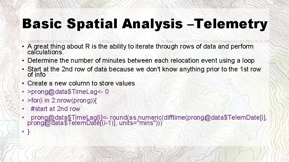
Basic Spatial Analysis –Telemetry • A great thing about R is the ability to iterate through rows of data and perform calculations. • Determine the number of minutes between each relocation event using a loop • Start at the 2 nd row of data because we don't know anything prior to the 1 st row of info • Create a new column to store values • >prong@data$Time. Lag<- 0 • >for(i in 2: nrow(prong)){ • #start at 2 nd row • prong@data$Time. Lag[i]<- round(as. numeric(difftime(prong@data$Telem. Date[i], prong@data$Telem. Date[(i-1)], units="mins"))) • }

Basic Spatial Analysis –Telemetry • Now value for 2 nd row to the first row >prong@data$Time. Lag[1]<- prong@data$Time. Lag[2] >View(prong@data) >str(prong@data)

Basic Spatial Analysis –Telemetry • Create a trajectory >l<- as. ltraj(xy=coordinates(prong), date=prong@data[, "Telem. Date"], id=prong@data[1, "ID__"], burst=prong@data[1, "ID__"]) >plot(l) • Convert trajetory to a line >tl<- ltraj 2 sldf(l) • Give it the same projection >proj 4 string(tl)<- proj 4 string(prong) >plot(tl) • Simplify the line >sl<- g. Simplify(tl, tol=6000) #rgeos package >plot(sl, add=TRUE, col="red")

Basic Spatial Analysis –Telemetry • Calculate home ranges • Start Minimum Convex Polygon (MCP) >cp 95 <- mcp(prong, percent = 95) • Plot the results >plot(pdem) >plot(prong, add=TRUE, col="green") >plot(cp 95, add=TRUE, border="red")

Other Useful Sites • Cheat Sheet http: //www. maths. lancs. ac. uk/~rowlings/Teaching/Use. R 2012/che atsheet. html • Spatial data with R http: //spatial. ly/r/ • CRAN: Analysis of Spatial Data http: //cran. r-project. org/web/views/Spatial. html • Maps with R http: //procomun. wordpress. com/2012/02/18/maps_with_r_1/