Basic Experimentation Notes developed by Ken Lulay Mechanical

Basic Experimentation Notes developed by Ken Lulay Mechanical Engineering University of Portland July 2008 (revised, September 2016) 1

Objectives n You will be able to: n Understand basic experiment “vocabulary” n Design and analyze a single variable experiment (2 level factor) n Design and analyze a multi-variable experiment (2 level factors) 2

Basic Experimentation - Overview n Experiment Basics n Single variable experiments – design and analysis n Multi-variable experiments – design and analysis 3

Overview of Experiment Basics n Differences between testing and experimenting n Experimental variables n Errors: systematic and random 4

Experimenting and testing… …both require obtaining data (taking measurements), but… …what are they and how are they different? 5

Testing n Testing may involve investigating only one set of conditions. n Usually evaluating performance n Example: determine strength of a material n May be a standardized test (ASMT, ISO) n Often has pass/fail criteria n Does it meet specifications or not? n We will not be discussing “testing” 6

Experimentation n Performed to increase knowledge n how things perform under differing conditions n Vary the input to determine the response n Requires more than one set of conditions (design points) n Evaluate “better/worse” (not pass/fail) 7

Experimentation & Testing A BIG difference: n Tests are often routine § Same tests done daily! § Analogous to daily commuting to work n Experiments are “unique” § Usually done only once! § Therefore, require more careful planning! § Analogous to a vacation trip 8

Variables n Variables are physical quantities that may or may not affect the results of an experiment or test. n Several types of variables are associated with any test and experiment: Controlled or Extraneous n n Controlled variable are held constant or intentionally manipulated (changed) during an experiment. Extraneous variables are not controlled. They are generally assumed to have no effect on the response (ex: ambient room temperature) 9

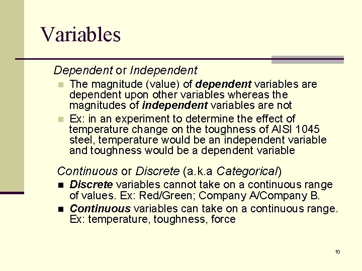
Variables Dependent or Independent n n The magnitude (value) of dependent variables are dependent upon other variables whereas the magnitudes of independent variables are not Ex: in an experiment to determine the effect of temperature change on the toughness of AISI 1045 steel, temperature would be an independent variable and toughness would be a dependent variable Continuous or Discrete (a. k. a Categorical) n n Discrete variables cannot take on a continuous range of values. Ex: Red/Green; Company A/Company B. Continuous variables can take on a continuous range. Ex: temperature, toughness, force 10

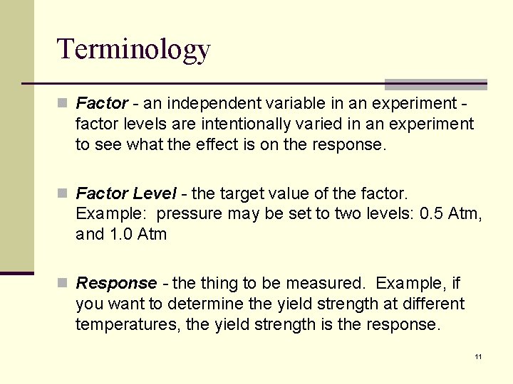
Terminology n Factor - an independent variable in an experiment - factor levels are intentionally varied in an experiment to see what the effect is on the response. n Factor Level - the target value of the factor. Example: pressure may be set to two levels: 0. 5 Atm, and 1. 0 Atm n Response - the thing to be measured. Example, if you want to determine the yield strength at different temperatures, the yield strength is the response. 11

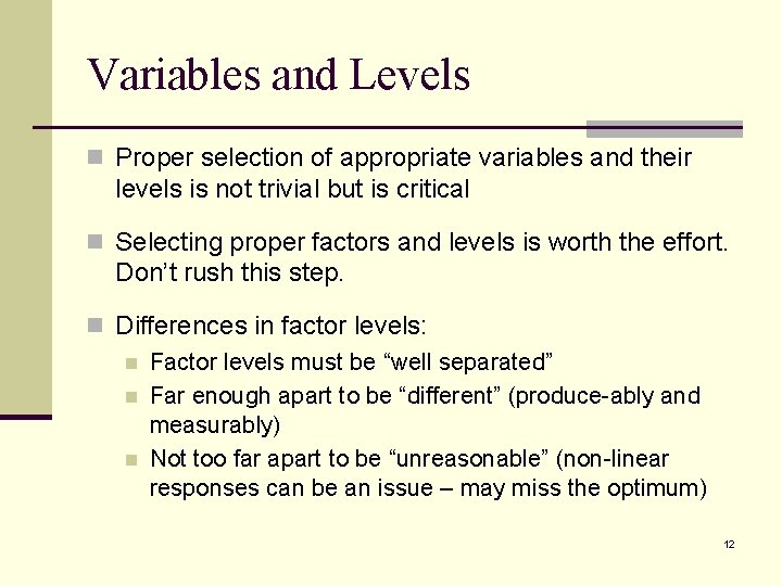
Variables and Levels n Proper selection of appropriate variables and their levels is not trivial but is critical n Selecting proper factors and levels is worth the effort. Don’t rush this step. n Differences in factor levels: n Factor levels must be “well separated” n Far enough apart to be “different” (produce-ably and measurably) n Not too far apart to be “unreasonable” (non-linear responses can be an issue – may miss the optimum) 12

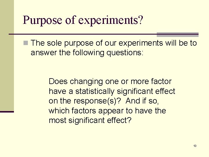
Purpose of experiments? n The sole purpose of our experiments will be to answer the following questions: Does changing one or more factor have a statistically significant effect on the response(s)? And if so, which factors appear to have the most significant effect? 13

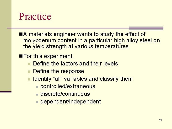
Practice n A materials engineer wants to study the effect of molybdenum content in a particular high alloy steel on the yield strength at various temperatures. n For this experiment: n n n Define the factors and their levels Define the response Identify “all” variables and classify them n controlled/extraneous n discrete/continuous n dependent/independent 14

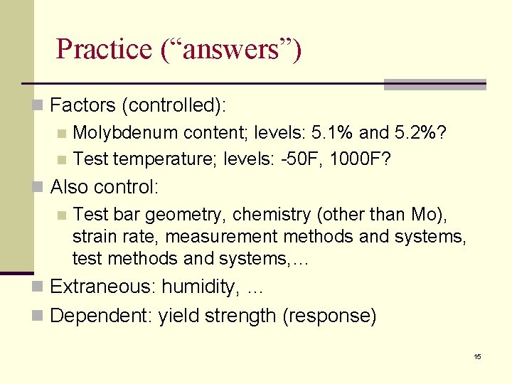
Practice (“answers”) n Factors (controlled): n Molybdenum content; levels: 5. 1% and 5. 2%? n Test temperature; levels: -50 F, 1000 F? n Also control: n Test bar geometry, chemistry (other than Mo), strain rate, measurement methods and systems, test methods and systems, … n Extraneous: humidity, … n Dependent: yield strength (response) 15

Errors (measurement variation) are due to a number of factors: n Measurement error n error = measured value - true value n Changes in test specimen n Ex: one specimen has slightly larger diameter n Changes in environment n Ex: ambient temperature increase n Et cetera 16

Errors n The “true” value is the value one would obtain with a perfect measurement. n The true value is never known in an experiment n Therefore, error can never be known exactly, it can only be estimated using statistical analysis. n Errors are inherent in measuring devices and caused by uncontrollable variations within the experiment. 17

Systematic and Random Errors In any experiment, two types of error can exist: n Systematic n Random 18

Systematic Errors n Caused by underlying factors which affect the results in a “consistent/reproducible” and sometime “knowable” way n Sometimes referred to as “bias” n Not random n DANGER: can lead to false conclusions! n Discuss this now, but example to follow later n Can be managed (reduced effects) by properly designed experiments (randomizing the test conditions). 19

Causes of Systematic Errors n Unknown changes during the experiment n temperature, procedures, equipment, etc. n Different batches of material or samples n Et cetera 20

Random Errors n Show no reproducible pattern – they are random. n Sometimes referred to as “noise. ” n Typically have normal distribution (bell shaped) averaging several readings can reduce random errors. 21

Practice n Consider the previous example (experiment to determine effect of varying molybdenum content and temperature on yield strength) n Make a list of possible systematic errors and random errors for the design on next slide… 22

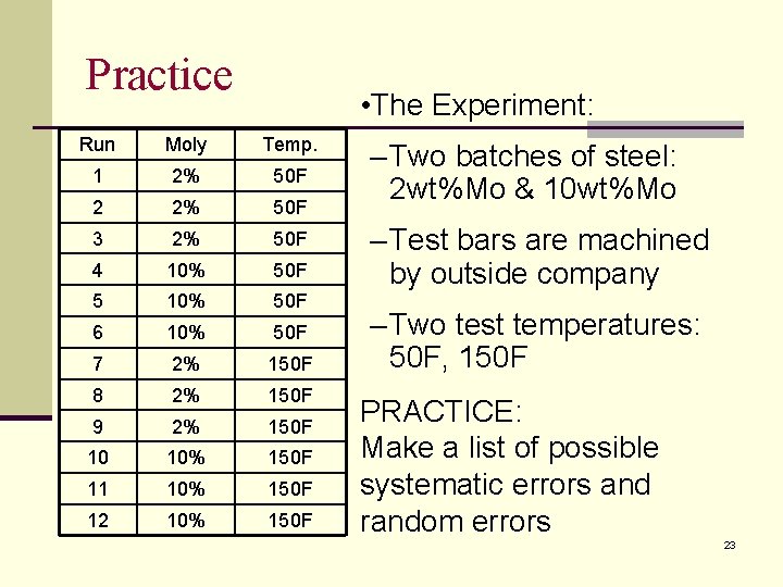
Practice • The Experiment: Run Moly Temp. 1 2% 50 F 2 2% 50 F 3 2% 50 F 4 10% 50 F 5 10% 50 F 6 10% 50 F 7 2% 150 F 8 2% 150 F 9 2% 150 F 10 10% 150 F 11 10% 150 F 12 10% 150 F – Two batches of steel: 2 wt%Mo & 10 wt%Mo – Test bars are machined by outside company – Two test temperatures: 50 F, 150 F PRACTICE: Make a list of possible systematic errors and random errors 23

Practice (“answers”) Possible systematic errors: n Batches of steel (chemistry variation of other elements) n n How could this effect be mitigated? Machining of specimens (did moly content affect machining quality? Were specimens machined in batches with different diameters? ) Temperature drift during testing (maybe from 52 F towards 48 F, and from 152 F towards 148)? Variation between beginning and end of test (measurement systems, operator, test equipment, test procedures…) How could systematic errors have been reduced? 24

Practice (“answers”) Possible random errors: Measurement errors n Diameter of bars (maybe random) n Load cell variation n Others? n 25

Review of Terminology n Do Exercise 1 (definitions). 26

Single Variable Experiments to follow 27

Overview of Single Variable Experiments n Basic Design of Experiments (DOE) n Example of “how not to” n Statistics and t-testing n Hypothesis testing n Confidence Intervals 28

Design of Experiments (DOE) n By careful design, errors can be mitigated n Systematic errors are mitigated by randomizing the test conditions (randomized run order) n Random errors are mitigated by increasing the number of data points n Design is a compromise of competing criteria: n Cost, time, availability of equipment, etc. n Control over variables n Importance of results and conclusion n CAREFUL PLANNING is REQUIRED! n Let’s look at a basic example… 29

Example: Single Variable Experiment n Wacky Engineer, a new employee at ASKO, believes that the color of paint applied to a tensile bar can affect the strength. n Let’s take a look at this experiment… 30

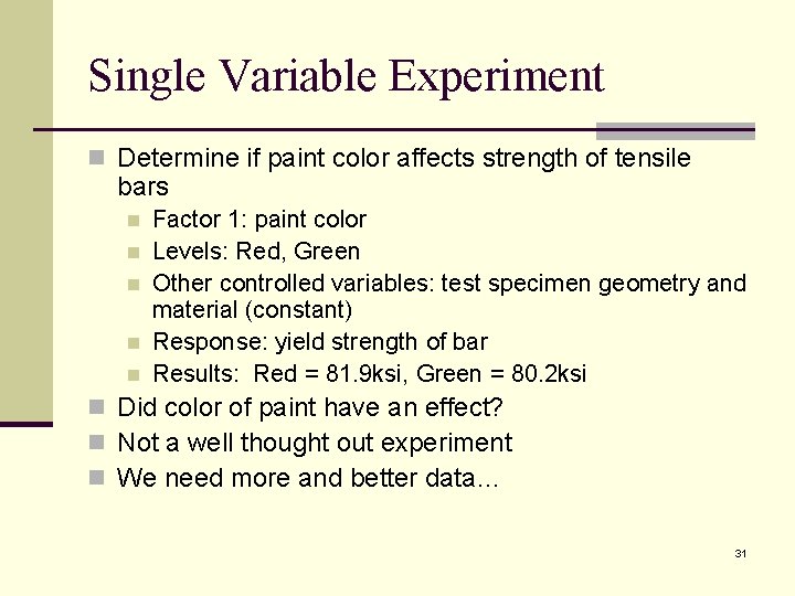
Single Variable Experiment n Determine if paint color affects strength of tensile bars n n n Factor 1: paint color Levels: Red, Green Other controlled variables: test specimen geometry and material (constant) Response: yield strength of bar Results: Red = 81. 9 ksi, Green = 80. 2 ksi n Did color of paint have an effect? n Not a well thought out experiment n We need more and better data… 31

Single Variable Experiment n New Experiment with more data: n paint five bars red and five green n Red paint is available, green paint is on backorder. n Your boss really wants data soon! n Test facility is available, so show progress: Paint and test red bars! n Green paint arrives, complete the testing! 32

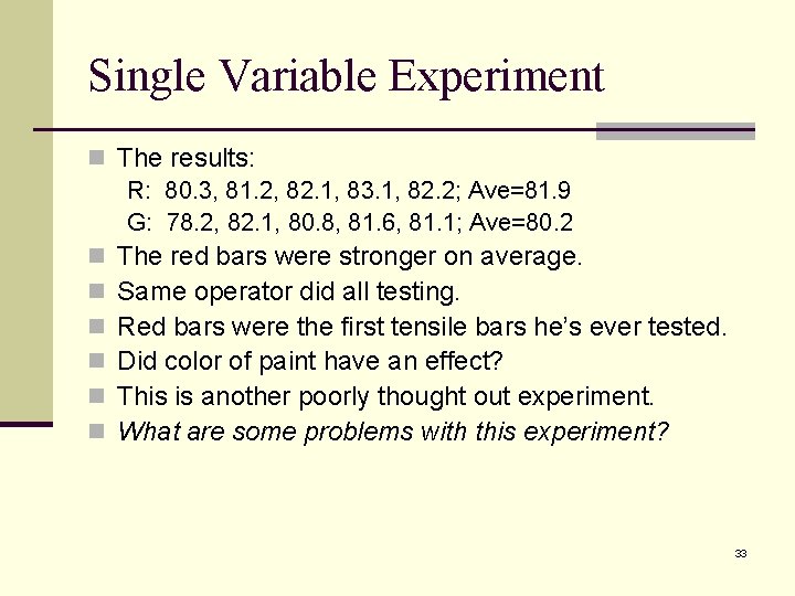
Single Variable Experiment n The results: R: 80. 3, 81. 2, 82. 1, 83. 1, 82. 2; Ave=81. 9 G: 78. 2, 82. 1, 80. 8, 81. 6, 81. 1; Ave=80. 2 n The red bars were stronger on average. n Same operator did all testing. n Red bars were the first tensile bars he’s ever tested. n Did color of paint have an effect? n This is another poorly thought out experiment. n What are some problems with this experiment? 33

Another, Better Example Re-do the prior experiment, but randomize n Randomize by using the following run order: n R, G, G, R, R, G, R n n why randomize? Why would the following run order not be “OK”? n R, G, R, G 34

Better Example n The randomized run order results: R: 80. 3, 81. 2, 82. 1, 83. 1, 82. 2; Ave=81. 9 G: 78. 2, 82. 1, 79. 8, 79. 6, 81. 1; Ave=80. 2 n R & G averages are different but did color of paint really have an effect? n Averages are only part of the answer n “Statistically significant” difference depends upon both the averages and the variation. 35

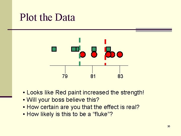
Plot the Data 79 81 83 • Looks like Red paint increased the strength! • Will your boss believe this? • How certain are you that the effect is real? • How likely is this to be a “fluke”? 36

n Need some statistical stuff… 37

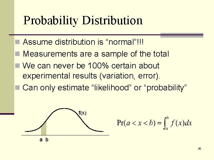
Probability Distribution n Assume distribution is “normal”!!! n Measurements are a sample of the total n We can never be 100% certain about experimental results (variation, error). n Can only estimate “likelihood” or “probability” f(x) a b 38

t-test n Comparing the averages is NOT sufficient! n The best way to answer “are they different” is with the t- test. n The t-test incorporates both the deviation of the data as well as the means. 39

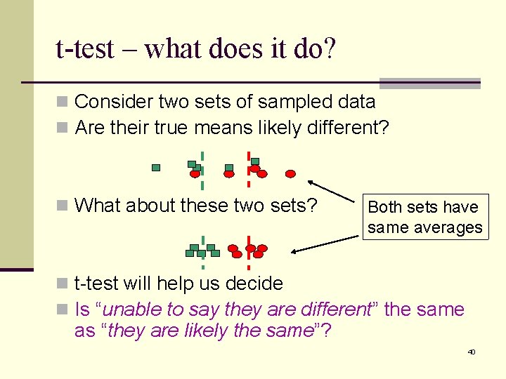
t-test – what does it do? n Consider two sets of sampled data n Are their true means likely different? n What about these two sets? Both sets have same averages n t-test will help us decide n Is “unable to say they are different” the same as “they are likely the same”? 40

Basic Statistics n n n m = true mean X = estimated mean based on finite sample size s = true standard deviation S = estimated standard deviated based on the finite sample size n = number of samples xi is the value of the ith sample (Equation 1) (Equation 2) 41

Basic Statistics, Continued n Note: X is an estimate of the actual mean (m). It becomes closer to m with increasing sample size, n. X itself is a random sample of the true mean, m (~central limit theorem). n For normally distributed data: 68. 3% of all data will be with in +/- 1 s 95. 4% of all data will be with in +/- 2 s 99. 7% of all data will be with in +/- 3 s 42

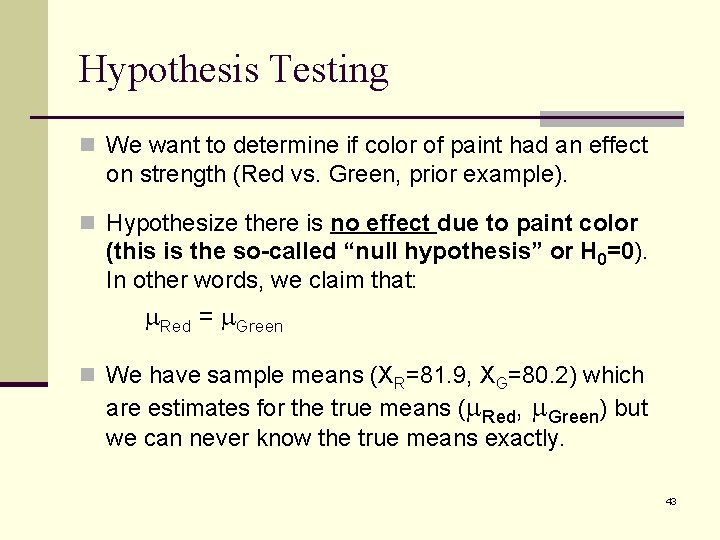
Hypothesis Testing n We want to determine if color of paint had an effect on strength (Red vs. Green, prior example). n Hypothesize there is no effect due to paint color (this is the so-called “null hypothesis” or H 0=0). In other words, we claim that: m. Red = m. Green n We have sample means (XR=81. 9, XG=80. 2) which are estimates for the true means (m. Red, m. Green) but we can never know the true means exactly. 43

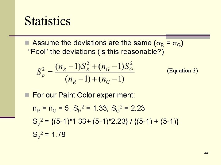
Statistics n Assume the deviations are the same (s. R = s. G) “Pool” the deviations (is this reasonable? ) (Equation 3) n For our Paint Color experiment: n. R = n. G = 5, SR 2 = 1. 33; SG 2 = 2. 23 Sp 2 = {(5 -1)*1. 33+ (5 -1)*2. 23} / {(5 -1) + (5 -1)} Sp 2 = 1. 78 44

t-test n We now define t 0, which is from the t-distribution (don’t worry about what “t-distribution” means): (Equation 4) n For our example: t 0 = ABS{81. 9 – 80. 2} / {1. 78 (1/5 + 1/5)}1/2 t 0 = 2. 06 45

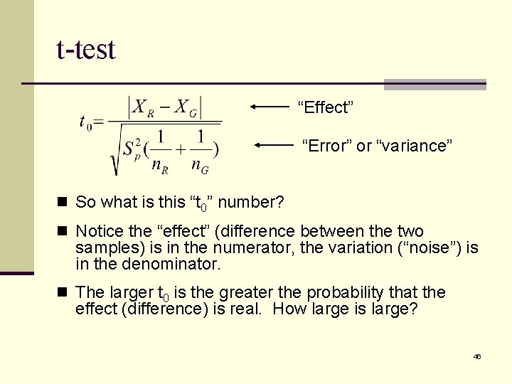
t-test “Effect” “Error” or “variance” n So what is this “t 0” number? n Notice the “effect” (difference between the two samples) is in the numerator, the variation (“noise”) is in the denominator. n The larger t 0 is the greater the probability that the effect (difference) is real. How large is large? 46

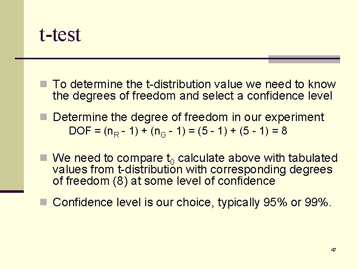
t-test n To determine the t-distribution value we need to know the degrees of freedom and select a confidence level n Determine the degree of freedom in our experiment DOF = (n. R - 1) + (n. G - 1) = (5 - 1) + (5 - 1) = 8 n We need to compare t 0 calculate above with tabulated values from t-distribution with corresponding degrees of freedom (8) at some level of confidence n Confidence level is our choice, typically 95% or 99%. 47

t-distribution Table n We select 95% confidence as our criterion n For 95% confidence interval, a = 0. 05 (= 1 - 0. 95) n There are 8 degrees of freedom in this experiment n From t-distribution: ta/2, DOF = t 0. 05/2, 8 = 2. 31 n t-distribution values are obtained from tables in most statistics/experimentation books. Note, ta/2 – means we are using 2 -sided or 2 -tailed test which is appropriate for the hypothesis of m. R =m. G because it is possible for m. R >m. G or m. R <m. G. If we were to ask the question is m. R > m. G, then we would use single-sided t-table (ta/1, DOF). 48

t-test n In our paint example t 0 < ta/2, DOF (2. 06 < 2. 31) n t 0 is too small to reject the null hypothesis at 95% confidence. n Therefore, do we accept the null hypothesis? (m. Red = m. Green). n This does not mean we are 95% confident that the bars painted red were equal to the green. It means we cannot say with confidence that they are different. Next slide… 49

95% Confident? “Cannot say they are different” is not equal to “saying they are the same”. RE: A “well mixed” box of 100 apples: any of the apples can be either red or green. Null Hypothesis: number of red = number of green n New box, pull 30 out: 1 is red, 29 are green – would you reject the null hypothesis? n Null hypothesis: number of red = number of green n New box, pull 30 apples out: 15 red, 15 are green – would you reject the null hypothesis? n Pull 99 apples: 49 are red, 50 are green…? 50

Exercise – t-test n Task: conduct an experiment to determine if there is a n n difference in the fatigue life between two brands of paperclips. Fatigue life is defined in this experiment as number of times the clip can be bent back and forth 90 degrees. One 90 degree bend is one fatigue cycle. If there are 10 or more people in the class, split the class in half (effectively conducting two identical experiments with about 5 data points per paperclip brand in each experiment). Each person in the class should break one of each brand record their results. Use the worksheets in back of this book. 51

Pairing – a special condition t-test n Determining relative magnitudes of the “effect” and “noise” is foundational for statistical analysis of experimental data. n “Noise” comes from many sources: differing batches of specimens, differing test or measurement apparatus, operator differences, etc. n If we can “filter out” noise, we would be able to perform a more effective analysis. 52

Pairing – a special condition t-test n If there is a single source of noise that we can identify and control, we may be able to “pair” the data. n For example, if we want to test the wear life of a new alloy, we may conduct an experiment to compare the life of the new alloy with a traditional alloy. n Put several of each part on buckets in the field. n Due to differing loading conditions, one would expect there to be large variability in wear from one bucket to another. Therefore, the bucket variation will introduce a large amount of noise. 53

Pairing – a special condition t-test n Pairing: put one sample of each alloy on each bucket (alternating location (left-right) of the two alloys from bucket to bucket). Determine the difference in life on each bucket between the two alloys. n Since each alloy on a given bucket presumably will experience similar loading, pairing will effectively “filter out” the noise contributed by bucket-to-bucket variation. n The null hypothesis now becomes m. D = 0, where m. D is the difference in means between the two groups (alloys, in this example). 54

Pairing – a special condition t-test For paired t-test where (Equation 5) XD is the average of the differences, n. D is the number of pairs of data, d i is the individual data (difference). 55

Exercise - Pairing n What about our paperclip experiment? n A potentially large source of error was operator-to-operator variability. n Each operator tested one of each paperclip, therefore, we can analyze using pairing! How lucky! n Using the worksheet in the back of this booklet, re-analyze the paperclip fatigue data using pairing (Exercise 3). 56

A bit more on pairing… n n n n n Situation: Your company produces optical supplies. The quality of optical mirrors is not satisfactory. You believe that the problem has to do with grinding speed. Given: *Your company has 12 grinding machines to produce optical mirrors. *The machines are numbered 1 -12, but are randomly placed throughout the shop. *You are allowed to use a total of 24 mirrors in your experiment. Task: Design an experiment (i. e. fill in the table below) to determine which cutting speed is better, Fast or Slow. At a maximum, you will have 24 runs. You are not trying to evaluate grinding machine performance, so you may use any number of grinding machines (1, 2, . . . 12). 57

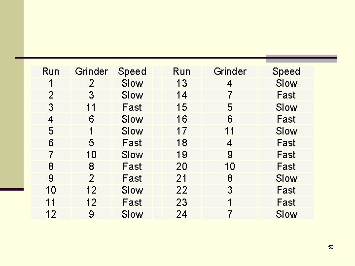
Run 1 2 3 4 5 6 7 8 9 10 11 12 Grinder 2 3 11 6 1 5 10 8 2 12 12 9 Speed Slow Fast Slow Fast Slow Run 13 14 15 16 17 18 19 20 21 22 23 24 Grinder 4 7 5 6 11 4 9 10 8 3 1 7 Speed Slow Fast Fast Slow 58

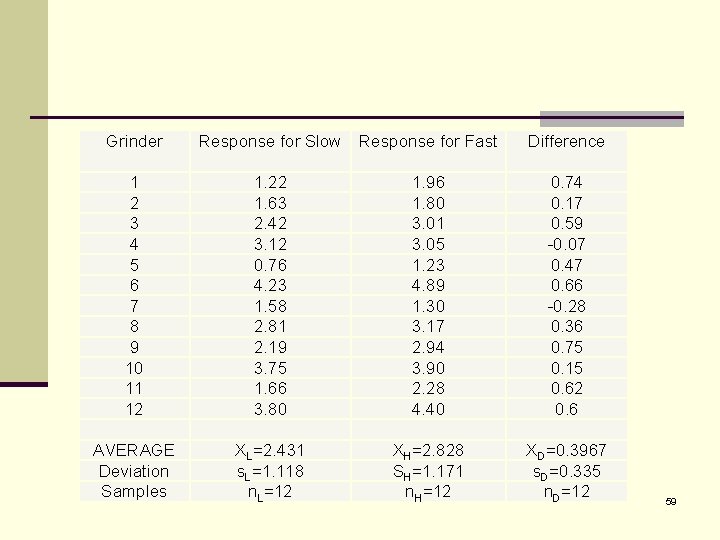
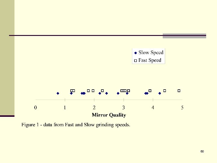
Grinder Response for Slow Response for Fast Difference 1 2 3 4 5 6 7 8 9 10 11 12 AVERAGE Deviation Samples 1. 22 1. 63 2. 42 3. 12 0. 76 4. 23 1. 58 2. 81 2. 19 3. 75 1. 66 3. 80 XL=2. 431 s. L=1. 118 n. L=12 1. 96 1. 80 3. 01 3. 05 1. 23 4. 89 1. 30 3. 17 2. 94 3. 90 2. 28 4. 40 XH=2. 828 SH=1. 171 n. H=12 0. 74 0. 17 0. 59 -0. 07 0. 47 0. 66 -0. 28 0. 36 0. 75 0. 15 0. 62 0. 6 XD=0. 3967 s. D=0. 335 n. D=12 59

60

61

Add 2 new data points created on one machine…do they appear to be “reasonable? ” 62

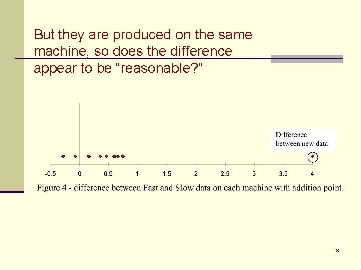
But they are produced on the same machine, so does the difference appear to be “reasonable? ” 63

Pairing – conclusion n Pairing is not always an option (need to be able to n n identify a single source of noise and then introduce one of each group to the precise same noise). If it is an option – do it! There is no cost other than planning for it. It will increase the power of the conclusion Not uncommon to fail to reject the null hypothesis using the t-test alone, but rejecting it using pairing analysis because of its increased power. 64

Can the t-test mislead us? n Yes! We can only make statements about probability! n Also, for the t-test to be valid, the data must have normal distribution. n There are two types of errors that can be made with hypothesis tests (next slide, please)… 65

Hypothesis Errors n Type I n The probability of erroneously rejecting the null hypothesis n Also known as the level of significance (equals a) n Type II n The probability of erroneously accepting the null hypothesis n The power of the experiment increases with increased number of data points (less likely to make a type II error) n These are independent, not complimentary (think about the previous “apple” example. ) 66

Confidence Intervals n Rather than asking the question “are they different” we may want to ask the question “how different are they” n Confidence Intervals help us answer that question 67

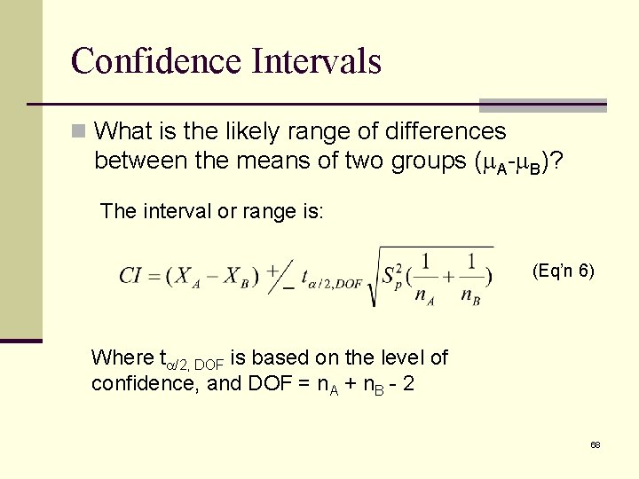
Confidence Intervals n What is the likely range of differences between the means of two groups (m. A-m. B)? The interval or range is: (Eq’n 6) Where ta/2, DOF is based on the level of confidence, and DOF = n. A + n. B - 2 68

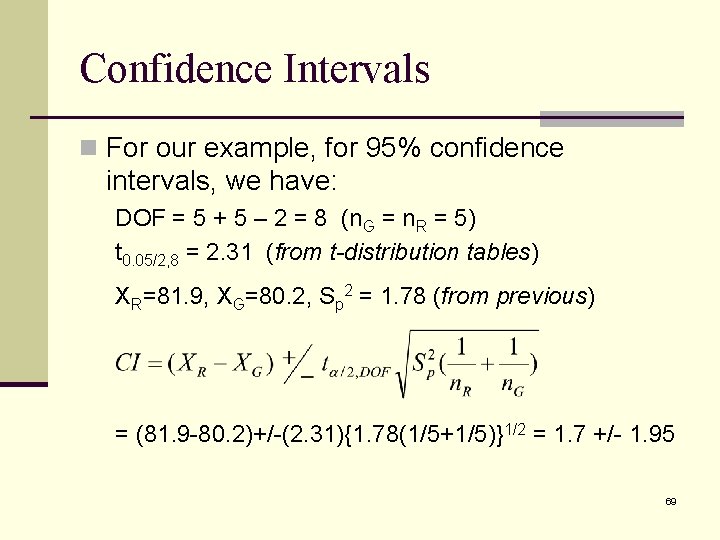
Confidence Intervals n For our example, for 95% confidence intervals, we have: DOF = 5 + 5 – 2 = 8 (n. G = n. R = 5) t 0. 05/2, 8 = 2. 31 (from t-distribution tables) XR=81. 9, XG=80. 2, Sp 2 = 1. 78 (from previous) = (81. 9 -80. 2)+/-(2. 31){1. 78(1/5+1/5)}1/2 = 1. 7 +/- 1. 95 69

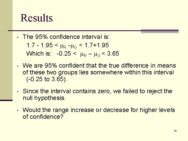
Results • The 95% confidence interval is: 1. 7 - 1. 95 < m. R -m. G < 1. 7+1. 95 Which is: -0. 25 < m. R – m. G < 3. 65 • We are 95% confident that the true difference in means of these two groups lies somewhere within this interval (-0. 25 to 3. 65). • Since the interval contains zero, we failed to reject the null hypothesis. • Would the range increase or decrease for higher levels of confidence? 70

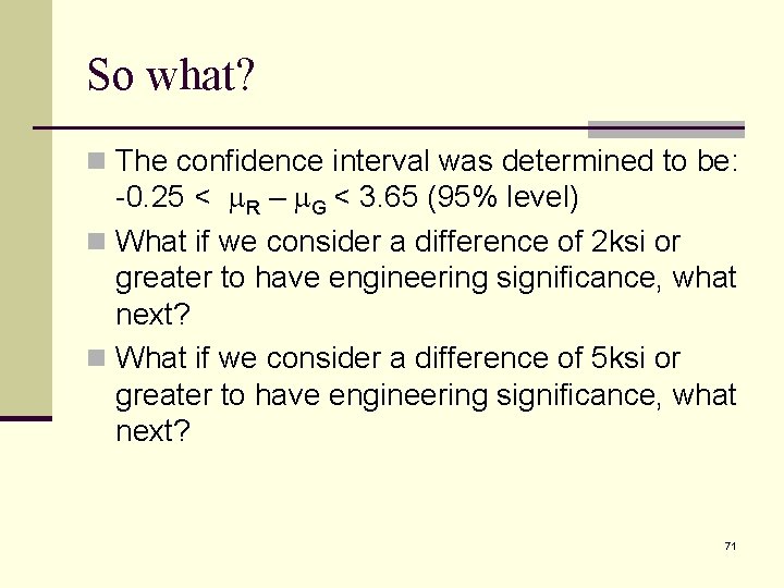
So what? n The confidence interval was determined to be: -0. 25 < m. R – m. G < 3. 65 (95% level) n What if we consider a difference of 2 ksi or greater to have engineering significance, what next? n What if we consider a difference of 5 ksi or greater to have engineering significance, what next? 71

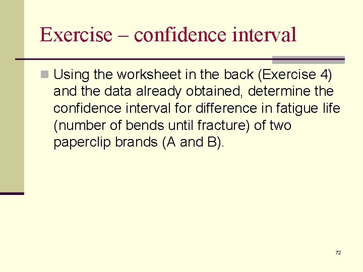
Exercise – confidence interval n Using the worksheet in the back (Exercise 4) and the data already obtained, determine the confidence interval for difference in fatigue life (number of bends until fracture) of two paperclip brands (A and B). 72

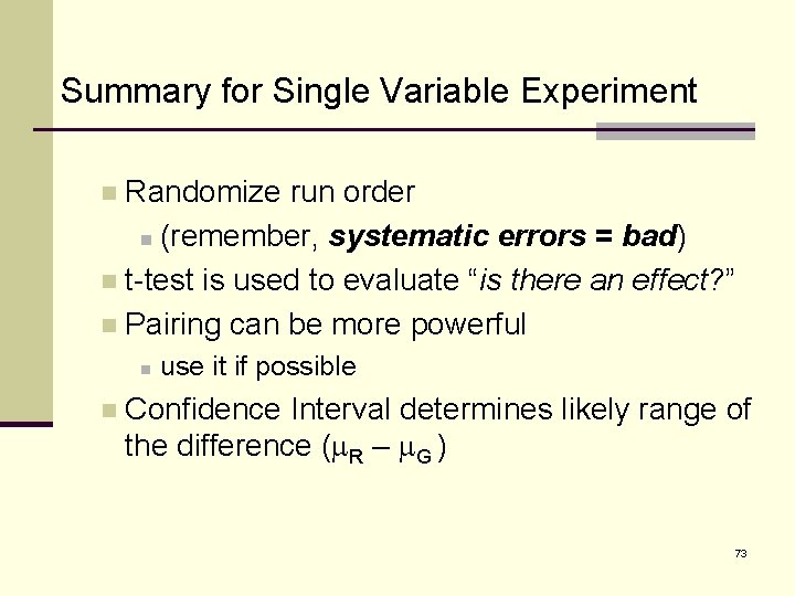
Summary for Single Variable Experiment Randomize run order n (remember, systematic errors = bad) n t-test is used to evaluate “is there an effect? ” n Pairing can be more powerful n n n use it if possible Confidence Interval determines likely range of the difference (m. R – m. G ) 73

What’s next? n We’ve looked at a single variable experiment. n What about more complicated conditions n experiments with two or more variables… 74

Multi-Variable Experiments to follow 75

Overview of Multi-Variable Experiments n “One variable at a time” approach n Interactions (what are they? ) n Terminology n Balanced design (what’s this? ) n Factorial Experiments n Practice (optimize a “manufacturing” process) 76

Purpose of experiments? n Remember, the purpose of experiments is to answer the question “does changing one or more factors have an effect on the response. ” n Our job is to answer that question using the limited resources available as well as possible. 77

Multi-Variables Using “One Variable at a Time” Approach n “One variable at a time” n Very basic experiment n Seems intuitive and simple n Reality: n Difficult to draw meaningful conclusions n Poor use of resources n Avoid these types of experiments! n Example to follow illustrates why 78

One Variable at a Time n Example: Determine optimal conditions for the following machining process: n Factors: Tool condition (levels: dull or sharp) n Cutting depth (levels: 0. 005” or 0. 010”) n Cutting speed (levels: 500 rpm and 1000 rpm) n n Response: surface finish 79

One Variable at a Time, Design n Test conditions: n Run 1, “baseline” or “control” n n Run 2, vary the tool condition n n dull, 0. 005”, 500 rpm Run 3: vary the depth n n sharp, 0. 005”, 500 rpm sharp, 0. 010”, 500 rpm Run 4: vary the speed n sharp, 0. 005”, 1000 rpm 80

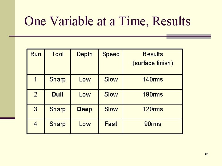
One Variable at a Time, Results Run Tool Depth Speed Results (surface finish) 1 Sharp Low Slow 140 rms 2 Dull Low Slow 190 rms 3 Sharp Deep Slow 120 rms 4 Sharp Low Fast 90 rms 81

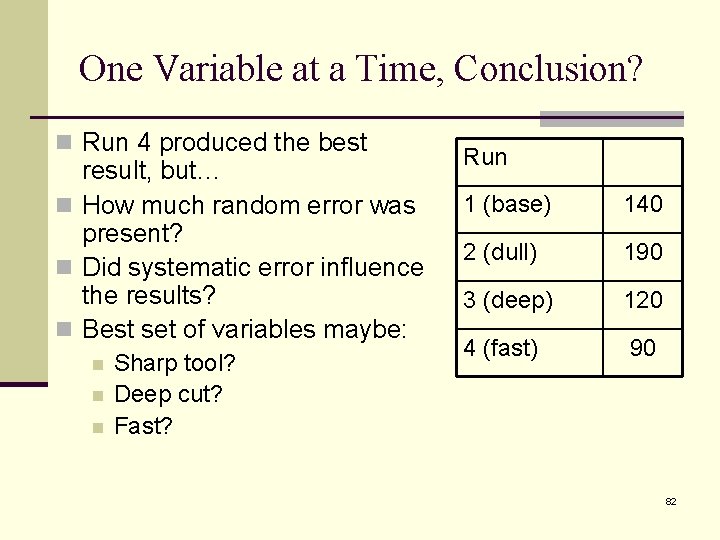
One Variable at a Time, Conclusion? n Run 4 produced the best result, but… n How much random error was present? n Did systematic error influence the results? n Best set of variables maybe: n n n Sharp tool? Deep cut? Fast? Run 1 (base) 140 2 (dull) 190 3 (deep) 120 4 (fast) 90 82

One Variable at a Time, Conclusion n We have only one data point for conditions of “dull”, “deep”, “fast”, but three data points for “sharp”, “low”, “slow” n There is no way to estimate errors (most conditions were tested only once) n Without estimating the errors, it is difficult to draw valid conclusions. n Did not test the “best conditions” together This is “okay” if there are no interactions n Could conduct another experiment to validate – but wouldn’t it have been better to do a complete job the first time? n 83

Interactions? We’ve identified that there are problems with the “one variable at a time” approach. Before considering better alternatives, we need to understand “interactions. ” 84

What are Interactions? n An interaction is when changing one factor influences how a different factor will affect the response. Clear? n Example: Conduct an experiment to determine which is more effective at keeping your shirt dry in the rain: an umbrella or a raincoat. n Experiment: 2 factors: n n n Factor 1, “weather”: rain with wind, rain with no wind Factor 2 , “tool”: umbrella, raincoat Response: “wetness” 85

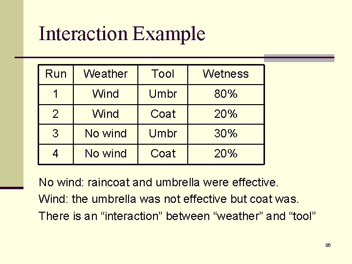
Interaction Example Run Weather Tool Wetness 1 Wind Umbr 80% 2 Wind Coat 20% 3 No wind Umbr 30% 4 No wind Coat 20% No wind: raincoat and umbrella were effective. Wind: the umbrella was not effective but coat was. There is an “interaction” between “weather” and “tool” 86

n What would no interaction “look like? ” n Contrast the previous with the following “no interaction” results… 87

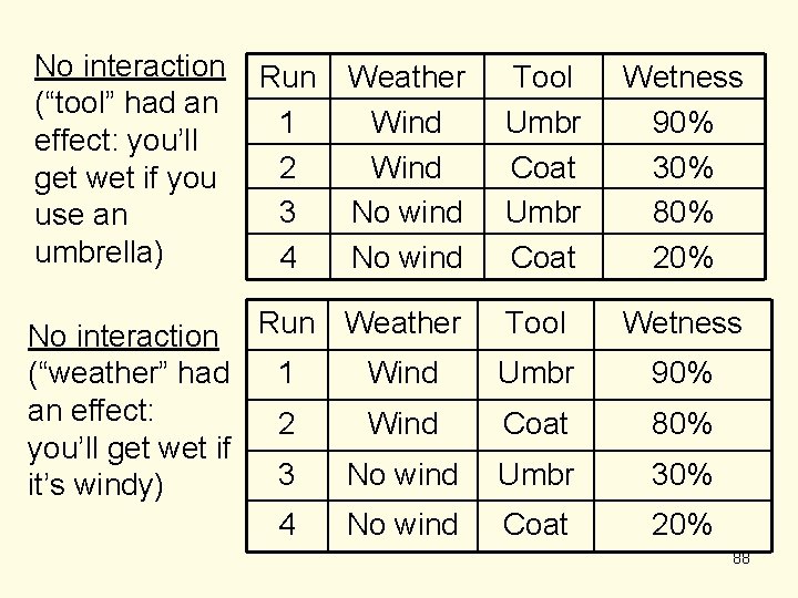
No interaction (“tool” had an effect: you’ll get wet if you use an umbrella) Run 1 2 3 4 Weather Wind No wind No interaction Run Weather (“weather” had 1 Wind an effect: 2 Wind you’ll get wet if 3 No wind it’s windy) 4 No wind Tool Umbr Coat Wetness 90% 30% 80% 20% Tool Wetness Umbr 90% Coat 80% Umbr 30% Coat 20% 88

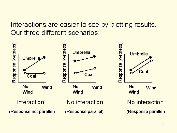
Umbrella Coat No Wind Interaction (Response not parallel) Umbrella Coat No Wind Response (wetness) Interactions are easier to see by plotting results. Our three different scenarios: Umbrella Coat No Wind No interaction (Response parallel) 89

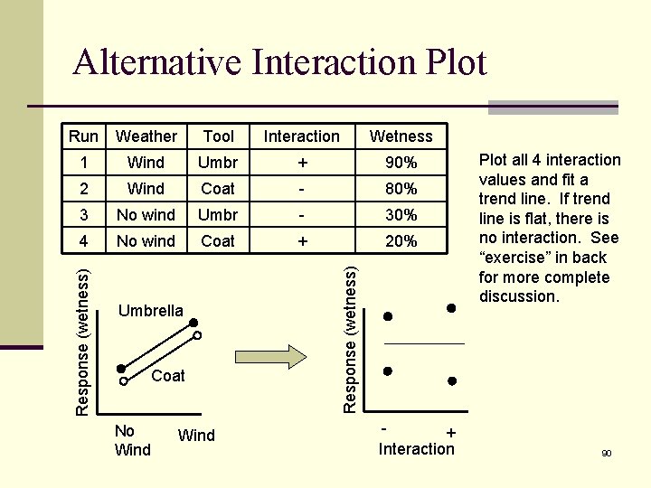
Alternative Interaction Plot Tool Interaction Wetness 1 Wind Umbr + 90% 2 Wind Coat - 80% 3 No wind Umbr - 30% 4 No wind Coat + 20% Umbrella Coat No Wind Response (wetness) Weather Response (wetness) Run + Interaction Plot all 4 interaction values and fit a trend line. If trend line is flat, there is no interaction. See “exercise” in back for more complete discussion. 90

Exercise - interactions Determine if interactions exist in the results shown in the exercise in the back of the booklet (Exercise 5). 91

End of Story for “One Variable at a Time” The “machining” example above did not evaluate interactions… …We can not determine what best set of conditions are. And not only are we not confident in the results, we have no idea of how “not confident” we are! 92

What’s next? n We’re almost ready for some really fun stuff… …but first, some terminology… …and then, explain what “balanced” designs mean. Then we can have fun with designing experiments “the right way!” 93

Terminology n Repetition - measuring the same response more than once (or taking another data point) without resetting up the experimental conditions. Decreases measurement errors to a limited degree. n Replication - requires completely redoing the experimental conditions. In other words, setting up the conditions as identically as possible to produce another measurement. n Very important to estimate the experimental error. n It shows the effects of set-up, and other unknown extraneous variables. n Replication is NOT the same as repetition, although they sound similar. 94

Terminology, cont. n Run - a set of experimental test conditions. All factors are set to specific levels. If I want to measure the boiling point at three pressure levels, I need at least three runs - one with the pressure at each of the 3 levels. n Treatment (design point) - a set of experimental conditions. One treatment is conducted each run, but treatments may be replicated in an experiment (may occur more than once). 95

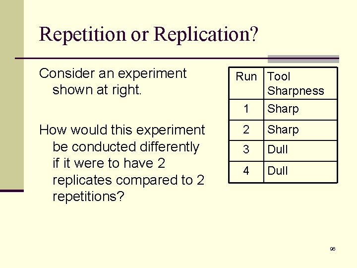
Repetition or Replication? Consider an experiment shown at right. How would this experiment be conducted differently if it were to have 2 replicates compared to 2 repetitions? Run Tool Sharpness 1 Sharp 2 Sharp 3 Dull 4 Dull 96

Designed Experiments (Design of Experiments, DOE’s) n Statistically based methodology of conducting and analyzing experiments n Interactions can be evaluated n Systematic error can be mitigated by randomization n Random error (noise) is mitigated by "balanced" designs since each variable is tested at different levels multiple times. n Let’s explain “balanced” design… 97

Balanced Design What it really means n Each factor is tested an equal number of times at n n each level For each factor setting, all of the other factors are set to each of their levels an equal number of times. The variation of all the other factors does not bias the results. Balanced designs do not necessarily test all possible conditions. Need an example to understand “balanced”… 98

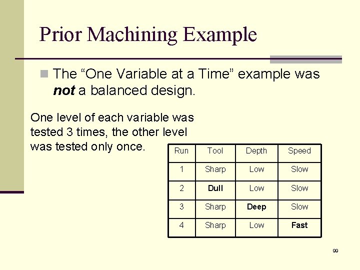
Prior Machining Example n The “One Variable at a Time” example was not a balanced design. One level of each variable was tested 3 times, the other level was tested only once. Run Tool Depth Speed 1 Sharp Low Slow 2 Dull Low Slow 3 Sharp Deep Slow 4 Sharp Low Fast 99

Example of Balanced Designs n Consider the “machining experiment”: n 3 factors, 2 levels each Tool: sharp, dull Depth: deep, low Speed: fast, slow n To run every possible combination would require 2 f runs where f is the number of factors (f=3, 23 = 8). n …but we don’t need all 8 conditions for a balanced design… n Balanced means…well, we need an example… 100

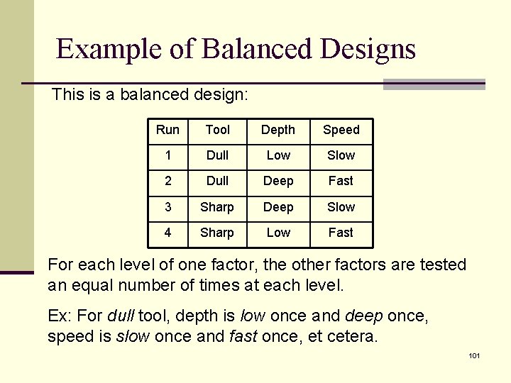
Example of Balanced Designs This is a balanced design: Run Tool Depth Speed 1 Dull Low Slow 2 Dull Deep Fast 3 Sharp Deep Slow 4 Sharp Low Fast For each level of one factor, the other factors are tested an equal number of times at each level. Ex: For dull tool, depth is low once and deep once, speed is slow once and fast once, et cetera. 101

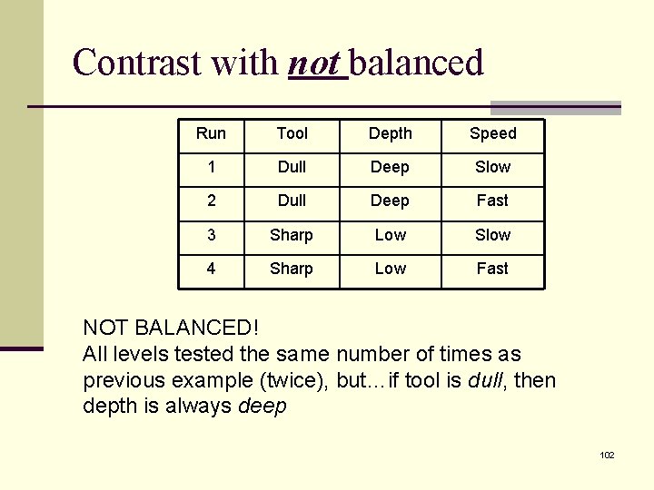
Contrast with not balanced Run Tool Depth Speed 1 Dull Deep Slow 2 Dull Deep Fast 3 Sharp Low Slow 4 Sharp Low Fast NOT BALANCED! All levels tested the same number of times as previous example (twice), but…if tool is dull, then depth is always deep 102

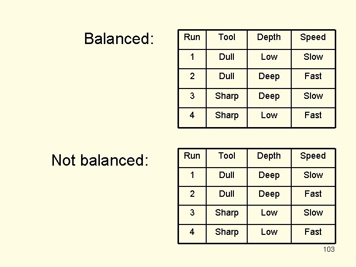
Balanced: Not balanced: Run Tool Depth Speed 1 Dull Low Slow 2 Dull Deep Fast 3 Sharp Deep Slow 4 Sharp Low Fast Run Tool Depth Speed 1 Dull Deep Slow 2 Dull Deep Fast 3 Sharp Low Slow 4 Sharp Low Fast 103

Exercise – balanced experiments Complete Exercise 6 in the back of this booklet: n Create a balanced experiment with two factors at two levels each. n n Assume 8 runs (22 = 4 conditions) Do not randomize (for this practice) n Factor A: levels: + and – n Factor B: levels: + and – n Notice “+” and “-” are often used in DOE’s to signify a “high” and “low” level. These are called “coded” levels 104

Review n We’ve studied Single Variable experiments (t-test, pairing, Confidence Intervals) n We have an understanding of interactions n We have an understanding of “balanced” design n We are ready to study experiments with multiple factors (factorial experiments) 105

Factorial Experiments – “The Right Way” n We will consider only full factorial experiments (experiments where all possible combinations are tested). n We will limit our discussion to experiments with two levels per factor. n Non-linear results will not be detected n The total number of possible combinations for experiments with multiple factors, all with two levels is 2 f, where f is the total number of factors (test variables). 106

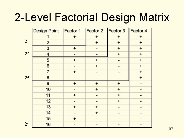
2 -Level Factorial Design Matrix 21 22 23 24 107

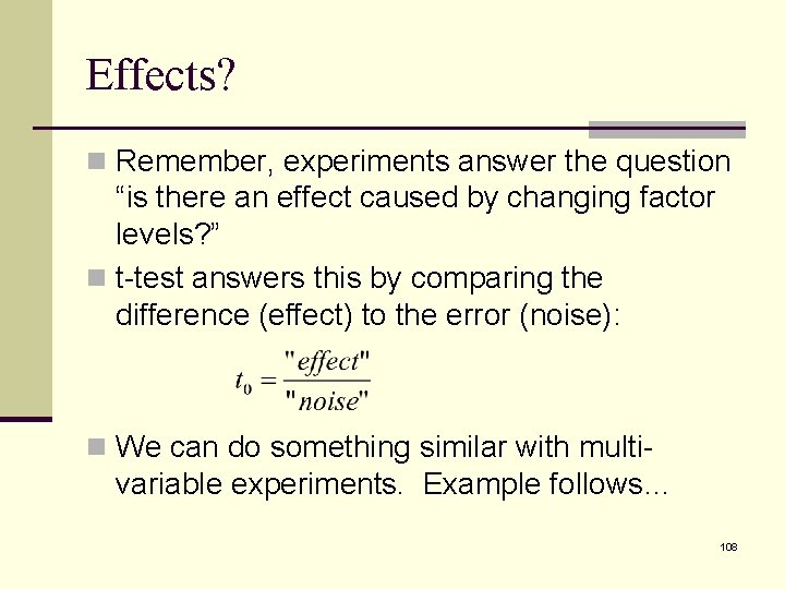
Effects? n Remember, experiments answer the question “is there an effect caused by changing factor levels? ” n t-test answers this by comparing the difference (effect) to the error (noise): n We can do something similar with multi- variable experiments. Example follows… 108

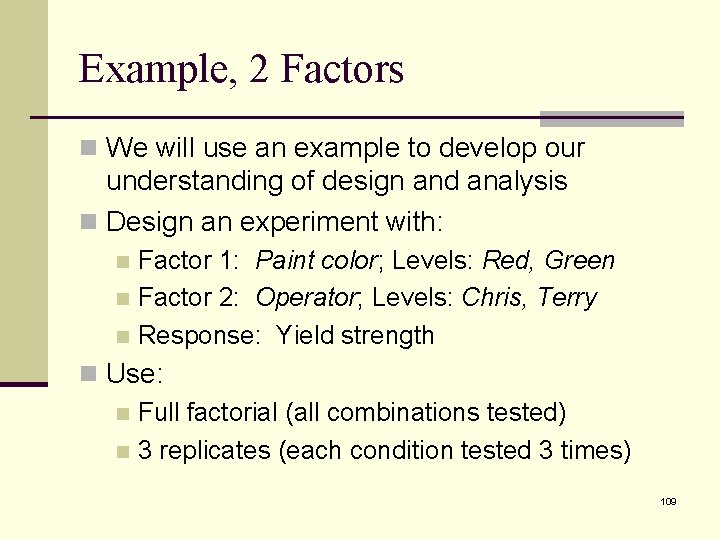
Example, 2 Factors n We will use an example to develop our understanding of design and analysis n Design an experiment with: Factor 1: Paint color; Levels: Red, Green n Factor 2: Operator; Levels: Chris, Terry n Response: Yield strength n n Use: n Full factorial (all combinations tested) n 3 replicates (each condition tested 3 times) 109

Design n To estimate error we need at least 2 replicates (each condition is tested twice) n More replicates = better estimate n We decide to have 3 replicates (each condition (design point) tested 3 times) n We need a balanced design 110

Design Matrix Design Point Factor 1 Factor 2 1 + + Red Chris 2 - + Green Chris 3 + - Red Terry 4 - - Green Terry (coded levels, +/-) Factor 1 Factor 2 (Non-coded levels) Factor 1, color: (+) = Red; (-) = Green Factor 2, operator: (+) = Chris; (-) = Terry 111

Interactions n With this DOE we will be able to analyze the effects of interactions. n Interactions are treated as an independent factors in the analysis n Two-way interactions (review): The effect of one factor depends upon the level of another n Ex: you will stay dry if you use an umbrella and no wind, but will stay dry if you use a raincoat regardless of wind. n 112

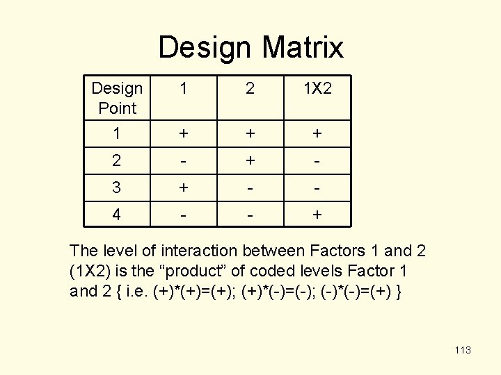
Design Matrix Design Point 1 1 2 1 X 2 + + + 2 - + - 3 + - - 4 - - + The level of interaction between Factors 1 and 2 (1 X 2) is the “product” of coded levels Factor 1 and 2 { i. e. (+)*(+)=(+); (+)*(-)=(-); (-)*(-)=(+) } 113

n The randomized run sheet is on next slide n Includes 3 replicates (each design point, or set of conditions, is tested 3 times) 114

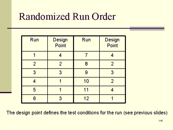
Randomized Run Order Run Design Point 1 4 7 4 2 2 8 2 3 3 9 3 4 1 10 2 5 1 11 4 6 3 12 1 The design point defines the test conditions for the run (see previous slides) 115

DOE Results n The experiment was conducted following the prescribed randomized run order. n The next slide shows the re-organized results and calculates the means n We will plot the results n Then we will step through the analysis… 116

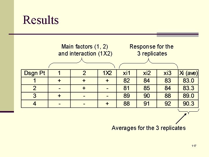
Results Main factors (1, 2) and interaction (1 X 2) Response for the 3 replicates Averages for the 3 replicates 117

n We are concerned with the averages, not the individual data points (they vary due to noise) n Let’s plot the data…graphs are a good way to visualize results… 118

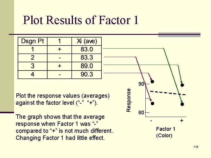
Plot Results of Factor 1 Plot the response values (averages) against the factor level (“-” “+”). The graph shows that the average response when Factor 1 was “-” compared to “+” is not much different. Changing Factor 1 had little effect. Response 90 80 - + Factor 1 (Color) 119

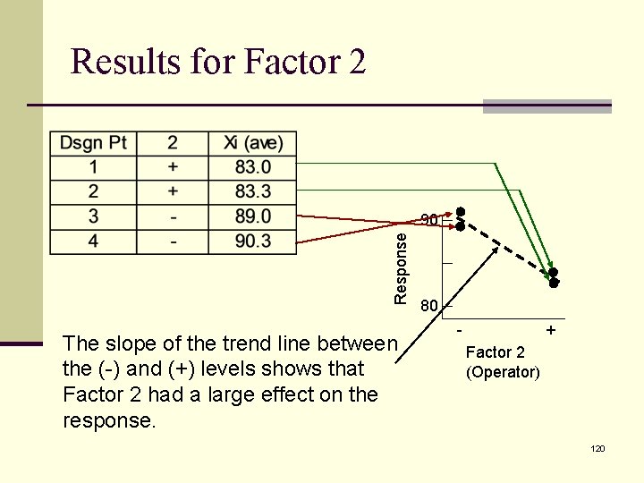
Results for Factor 2 Response 90 The slope of the trend line between the (-) and (+) levels shows that Factor 2 had a large effect on the response. 80 - + Factor 2 (Operator) 120

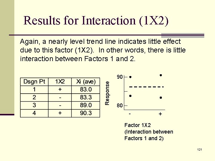
Results for Interaction (1 X 2) Again, a nearly level trend line indicates little effect due to this factor (1 X 2). In other words, there is little interaction between Factors 1 and 2. Response 90 80 - + Factor 1 X 2 (Interaction between Factors 1 and 2) 121

More Rigor (Statistics!) n The graphs are useful in terms of giving us a qualitative sense of effects. n But as we’ve seen, “averages” are not sufficient. n We need a method to quantify our confidence in the effect. n Where are we going? t-test is where! 122

Remember the “t-test”? n The t-test is used to answer the critical question: is there a statistically significant effect or is the change caused by random noise? n In order to answer that question in any experiment, we must compare the “effect” with the “noise. ” n We must determine both “effect” and “noise” n We’ll start with “noise” (error). 123

Nomenclature Let xij be the response of the jth replicate of treatment “i” Let Xi be the average of all responses within the replicate “j” Let XT be the average of all responses, total Let k be the total number of test conditions (design points) “i” goes from 1 to k. Let ni be the number of replicates for treatment “i”. Let N be the total number of tests 124

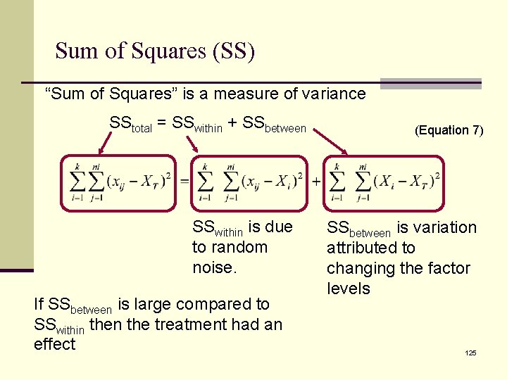
Sum of Squares (SS) “Sum of Squares” is a measure of variance SStotal = SSwithin + SSbetween SSwithin is due to random noise. If SSbetween is large compared to SSwithin the treatment had an effect (Equation 7) SSbetween is variation attributed to changing the factor levels 125

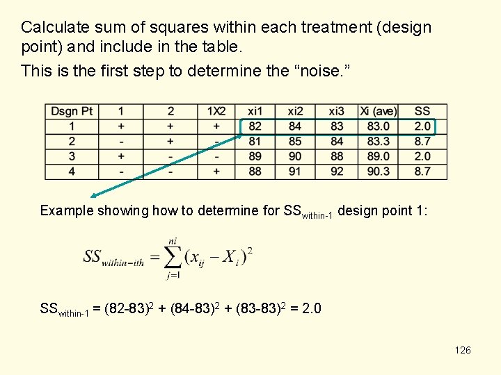
Calculate sum of squares within each treatment (design point) and include in the table. This is the first step to determine the “noise. ” Example showing how to determine for SSwithin-1 design point 1: SSwithin-1 = (82 -83)2 + (84 -83)2 + (83 -83)2 = 2. 0 126

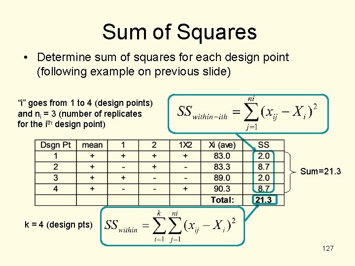
Sum of Squares • Determine sum of squares for each design point (following example on previous slide) “i” goes from 1 to 4 (design points) and ni = 3 (number of replicates for the ith design point) Sum=21. 3 k = 4 (design pts) 127

Experimental “noise” n SSwithin (calculated above) is related to the experimental “noise”, but it is not what we use in the t-test. n What do we use? n Next slide please… 128

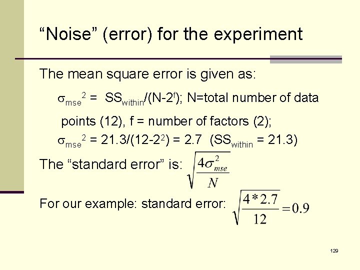
“Noise” (error) for the experiment The mean square error is given as: smse 2 = SSwithin/(N-2 f); N=total number of data points (12), f = number of factors (2); smse 2 = 21. 3/(12 -22) = 2. 7 (SSwithin = 21. 3) The “standard error” is: For our example: standard error: 129

“Noise” (error) for the experiment n The standard error (just calculated) is the same for all factors in the experiment – it is the “experimental noise. ” n Remember, t 0 is the ratio between “effect” and “noise” t 0 = effect / standard error 130

Effect We’ve determined the standard error But what was the effect of various factor levels? n Determine the average response for each factor at each level: Determine the average response when factor 1 was (+) and also when it was (-), then do this for factor 2, etc. n This procedure requires a balanced design n 131

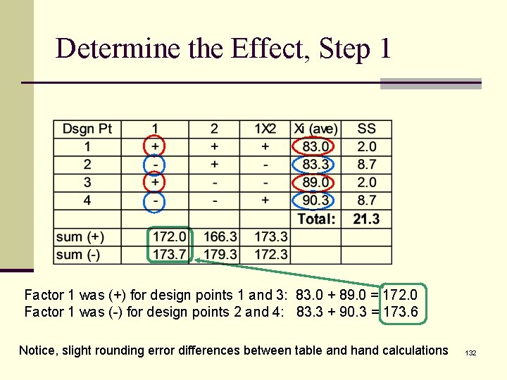
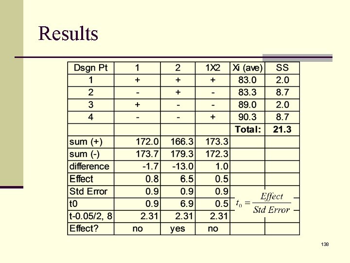
Determine the Effect, Step 1 Factor 1 was (+) for design points 1 and 3: 83. 0 + 89. 0 = 172. 0 Factor 1 was (-) for design points 2 and 4: 83. 3 + 90. 3 = 173. 6 Notice, slight rounding error differences between table and hand calculations 132

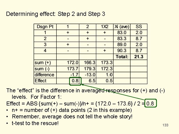
Determining effect: Step 2 and Step 3 The “effect” is the difference in averaged responses for (+) and (-) levels. For Factor 1: Effect = ABS {sum(+) – sum(-)}/n+ = {172. 0 – 173. 6} / 2 = 0. 8 • n+ = number of (+) data points (2 in this example) • Remember, average does not tell the whole story! • t-test to the rescue! 133

t-test Review § t 0 is the ratio of the “effect” to the “noise”. The larger t 0 is the greater the probability that the factor had a real effect. § In the previous table we calculated the effect of all three factors (1, 2, 1 X 2). The “effect” is the difference in averaged responses for (+) and (-) levels. § The noise has already been determined for our example (“standard error”). 134

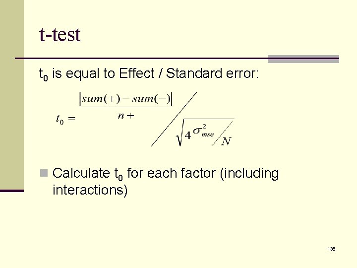
t-test t 0 is equal to Effect / Standard error: n Calculate t 0 for each factor (including interactions) 135

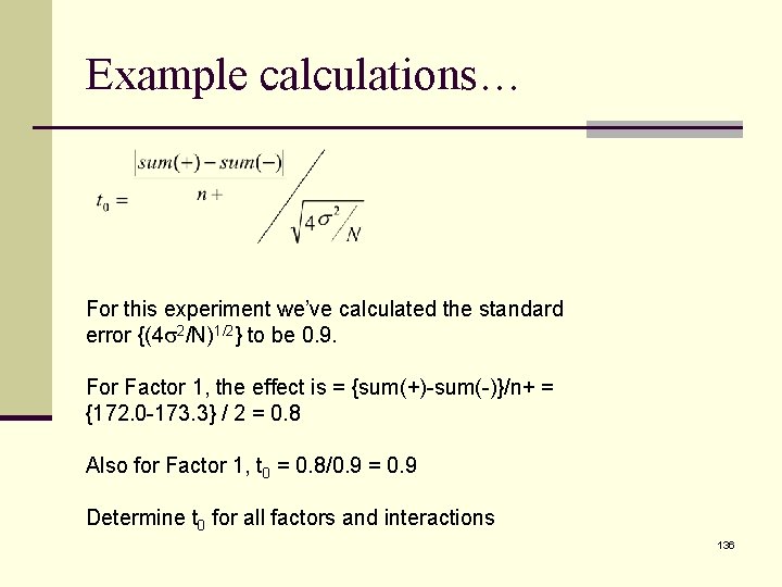
Example calculations… For this experiment we’ve calculated the standard error {(4 s 2/N)1/2} to be 0. 9. For Factor 1, the effect is = {sum(+)-sum(-)}/n+ = {172. 0 -173. 3} / 2 = 0. 8 Also for Factor 1, t 0 = 0. 8/0. 9 = 0. 9 Determine t 0 for all factors and interactions 136

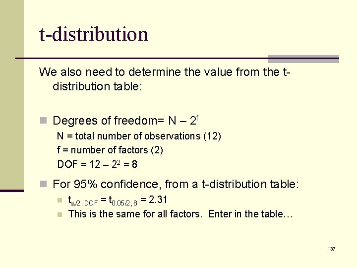
t-distribution We also need to determine the value from the tdistribution table: n Degrees of freedom= N – 2 f N = total number of observations (12) f = number of factors (2) DOF = 12 – 22 = 8 n For 95% confidence, from a t-distribution table: n n ta/2, DOF = t 0. 05/2, 8 = 2. 31 This is the same for all factors. Enter in the table… 137

Results 138

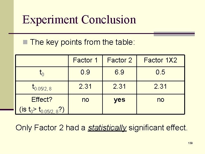
Experiment Conclusion n The key points from the table: Factor 1 Factor 2 Factor 1 X 2 t 0 0. 9 6. 9 0. 5 t 0. 05/2, 8 2. 31 Effect? (is t 0> t 0. 05/2, 8? ) no yes no Only Factor 2 had a statistically significant effect. 139

Factorial Experiment, Conclusion n The above example shows the basics of analyzing a factorial experiment. n DOE software will perform the analysis for you. n Usually, F-test is performed rather than ttest, but the concept is the same (they are equivalent). n We will do an experiment for practice, first, let’s talk about other aspects of an experiment… 140

Planning an Experiment n Okay, we now have some idea about DOE n “Design” is only a small part of the picture n To conduct an experiment properly, much more is required. This typically includes most of the following… 141

Experiment Process n Define the problem (write down a problem statement), n n define the objective (purpose). Determine available resources Determine factors, levels, and response(s) Create the design (number of runs, run order, etc. ) Obtain resources n $$$, measurement and test equipment, test specimens (have spares), personnel, etc. n Create a plan n Determine schedule for personnel, equipment, etc. n Create a run-sheet. n Save all used specimens, identify them. You may need to take another closer look at them later. 142

Practice Experiment n Problem: we like “good” popcorn – and we currently can’t make good popcorn. n Create an experiment to help solve this problem. n As a class, complete the next slide 143

Practice As a class: n Write a problem statement n Write clear objective of experiment n Determine Factors – only two – think carefully about what you select. n Determine factor levels (do not worry that some combination of factor levels will produce bad popcorn – this is to be expected) n Determine response (may be more than 1). Next slide please… 144

Practice n Factors you may have considered: n Time n Power setting n Placement of bag within the microwave n Orientation of the bag n Brands of popcorn n Different microwaves n Are “time” and “power setting” independent? Could they be combined and called “energy input”? n Resources are limited – we want the most useful information possible. 145

Exercise – full factorial experiment n Break into smaller groups (about 5 per group) and design and conduct the experiment and analyze the results. Use the worksheet in the back of this booklet (Exercise 7). n After completion, discuss as a class. 146

One last thing “Outliers” may be an issue in an experiment. Unfortunately, if only 1 or 2 data points are observed for a given set of experimental conditions, it is not possible to determine if an outlier exists. Even more detrimental, with few data points a single outlier can dramatically change the sample mean! What to do? Always do a “reality check” – do the results seem reasonable? If not, it may be due to an outlier – OR it may not be a error in any form (your judgment may be off – no shame in being surprised by results). Be careful about dismissing what you think is an outlier – it may not be! 147

Limitations to what we’ve done n We considered only experiments with: n n Assumed normal distributions All factors at 2 levels each n n These factors can be discrete or continuous Response must be continuous, not discrete At least 2 replicates n We did not look at “censored” data (such as fatigue data that is terminated after so many cycles even if there was no failure) n All Design Points were replicated an equal number of times n Full factorial (all possible combinations were tested) n Next slide please… n 148

Advanced Stuff – But Not Here, Not Now There are more advanced concepts (and surprisingly, these are not necessarily much more complicated to design or analyze. ) 149

Life beyond this course n Experiments do not actually require having a second replicate to estimate errors (talk to a statistician) n Fractionated experiments – experiments that not all possible combinations are tested. n n These are very beneficial if there is a large number of factors (2 f gets big fast!). The “cost” is lost knowledge regarding interactions. n Experiments can model non-linearity if more than 2 levels per factor are included 150

CONCLUSIONS n Experiments require planning! n Randomize to mitigate systematic errors n No pain, no gain n Select factors and their levels carefully n May want to “try out” levels (pre-experiment) before beginning a DOE n t-test helps answer “is there an effect” n Pairing is a good thing – if possible n Full factorial designs are effective and efficient for multi-variable experiments 151

Happy Experimenting! 152

Addendum to notes n ANOVA – Analysis of variation. This is the statistical heart of DOE’s. Typically uses ttest, or f-test to determine if there is an effect caused by changing factor levels. n f-test may be used to reject the null hypothesis for 2 or more groups. t-test may be used to reject the null hypothesis for 2 groups. 153

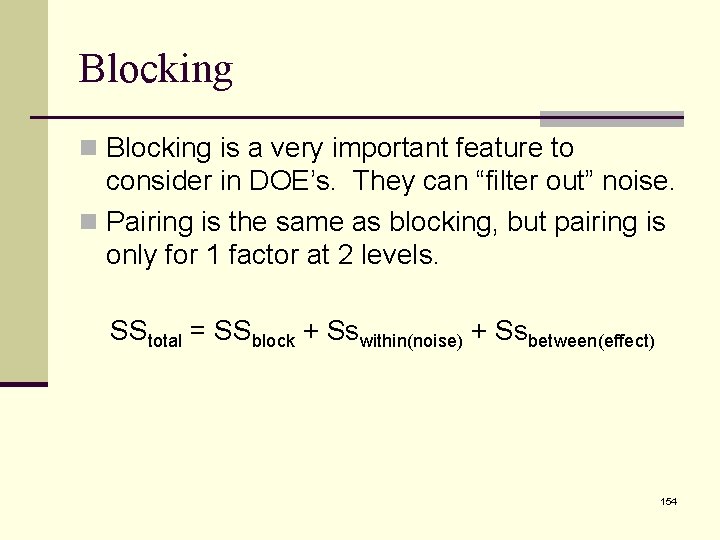
Blocking n Blocking is a very important feature to consider in DOE’s. They can “filter out” noise. n Pairing is the same as blocking, but pairing is only for 1 factor at 2 levels. SStotal = SSblock + Sswithin(noise) + Ssbetween(effect) 154

Reference n Most statistics books – especially those written for engineers. n Many books written on DOE’s specifically Online: n http: //onlinestatbook. com/2/analysis_of_varia nce/one-way. html 155