Basic Concepts in Control 393 R Autonomous Robots

Basic Concepts in Control 393 R: Autonomous Robots Peter Stone Slides Courtesy of Benjamin Kuipers

Good Afternoon Colleagues • Are there any questions?

Logistics • Reading responses • Next week’s readings - due Monday night – Braitenberg vehicles – Forward/inverse kinematics – Aibo joint modeling • Next class: lab intro (start here)

Controlling a Simple System • Consider a simple system: – Scalar variables x and u, not vectors x and u. – Assume x is observable: y = G(x) = x – Assume effect of motor command u: • The setpoint xset is the desired value. – The controller responds to error: e = x xset • The goal is to set u to reach e = 0.

The intuition behind control • Use action u to push back toward error e = 0 – error e depends on state x (via sensors y) • What does pushing back do? – Depends on the structure of the system – Velocity versus acceleration control • How much should we push back? – What does the magnitude of u depend on? Car on a slope example

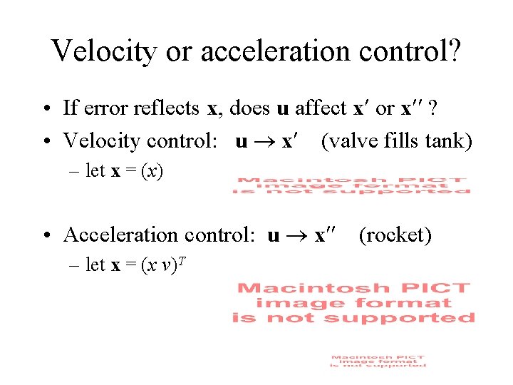
Velocity or acceleration control? • If error reflects x, does u affect x or x ? • Velocity control: u x (valve fills tank) – let x = (x) • Acceleration control: u x (rocket) – let x = (x v)T

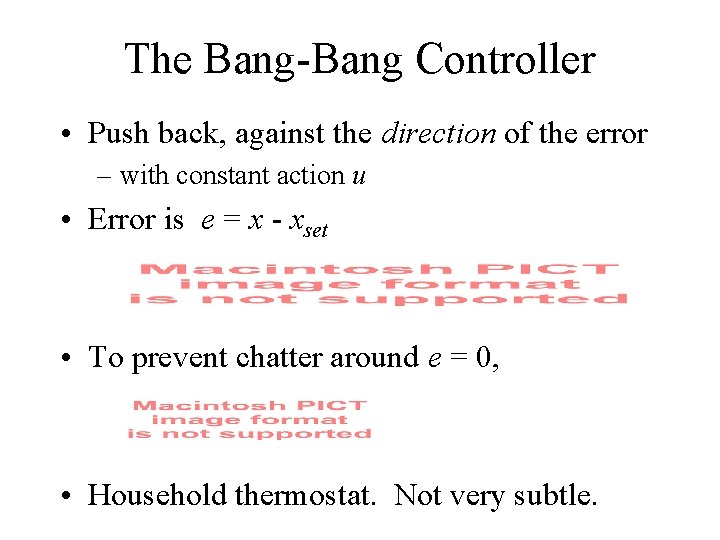
The Bang-Bang Controller • Push back, against the direction of the error – with constant action u • Error is e = x - xset • To prevent chatter around e = 0, • Household thermostat. Not very subtle.

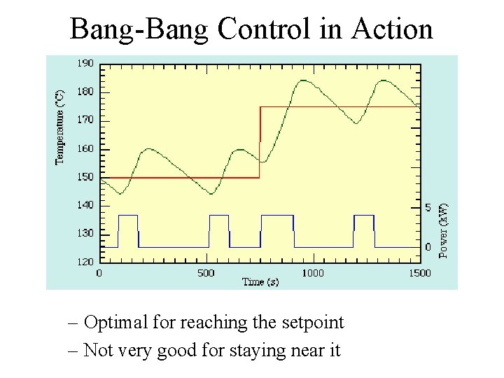
Bang-Bang Control in Action – Optimal for reaching the setpoint – Not very good for staying near it

Hysteresis • Does a thermostat work exactly that way? – Car demonstration • Why not? • How can you prevent such frequent motor action? • Aibo turning to ball example

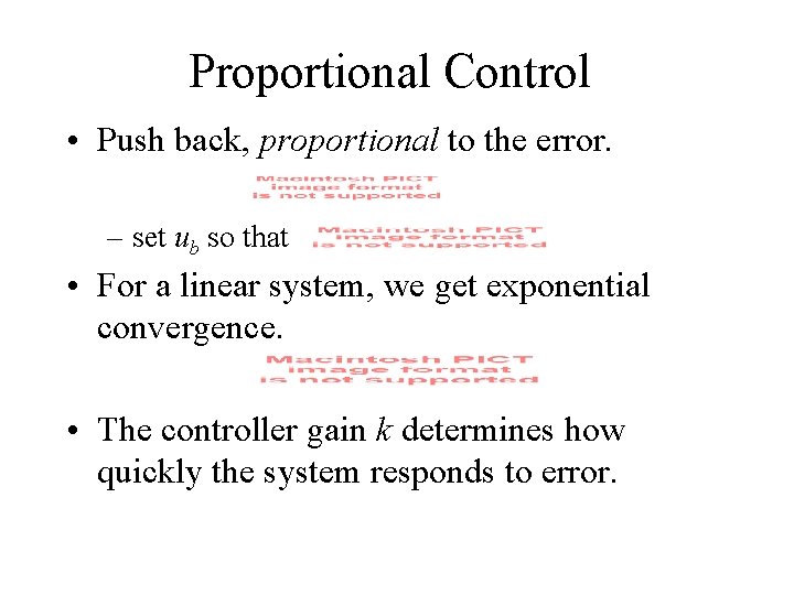
Proportional Control • Push back, proportional to the error. – set ub so that • For a linear system, we get exponential convergence. • The controller gain k determines how quickly the system responds to error.

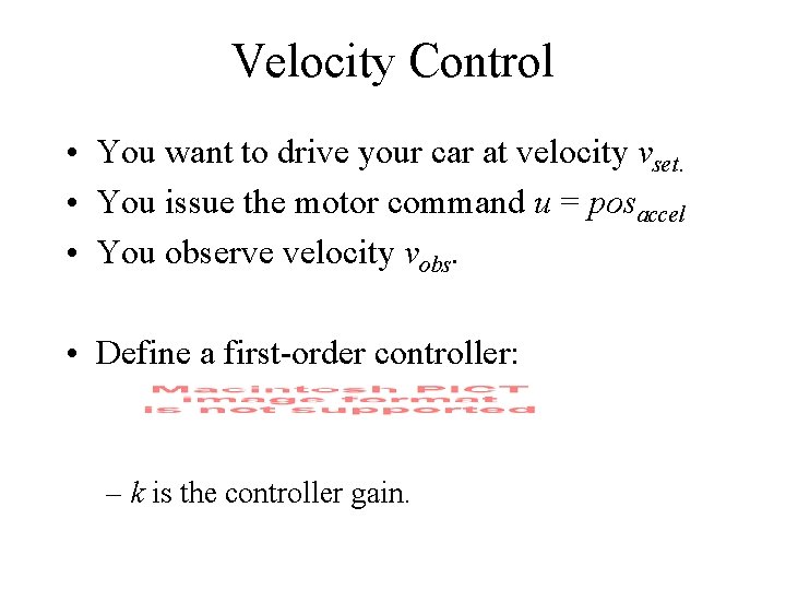
Velocity Control • You want to drive your car at velocity vset. • You issue the motor command u = posaccel • You observe velocity vobs. • Define a first-order controller: – k is the controller gain.

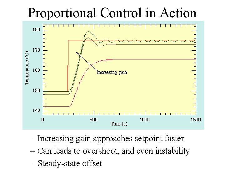
Proportional Control in Action – Increasing gain approaches setpoint faster – Can leads to overshoot, and even instability – Steady-state offset

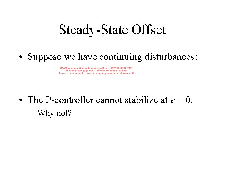
Steady-State Offset • Suppose we have continuing disturbances: • The P-controller cannot stabilize at e = 0. – Why not?

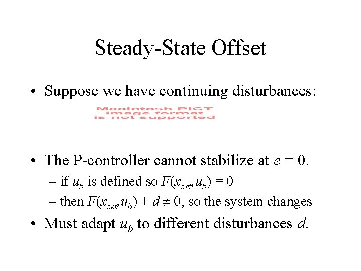
Steady-State Offset • Suppose we have continuing disturbances: • The P-controller cannot stabilize at e = 0. – if ub is defined so F(xset, ub) = 0 – then F(xset, ub) + d 0, so the system changes • Must adapt ub to different disturbances d.

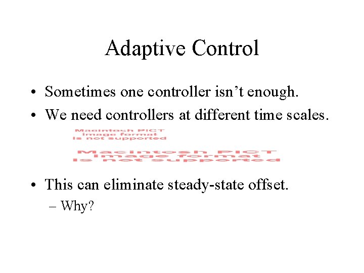
Adaptive Control • Sometimes one controller isn’t enough. • We need controllers at different time scales. • This can eliminate steady-state offset. – Why?

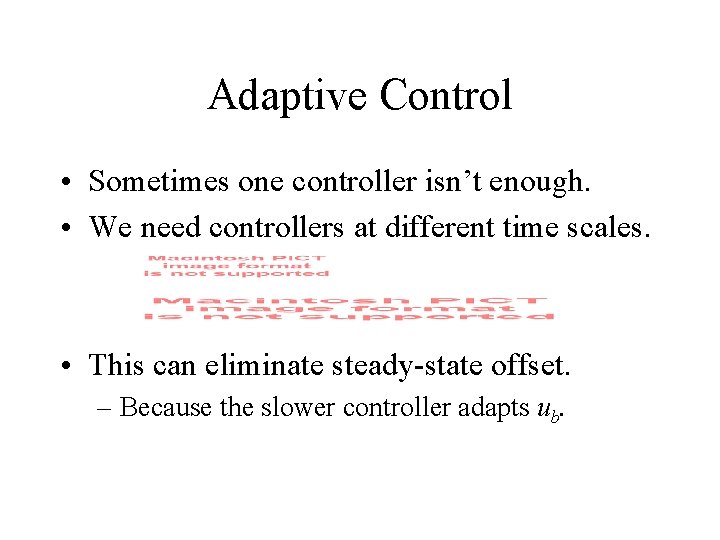
Adaptive Control • Sometimes one controller isn’t enough. • We need controllers at different time scales. • This can eliminate steady-state offset. – Because the slower controller adapts ub.

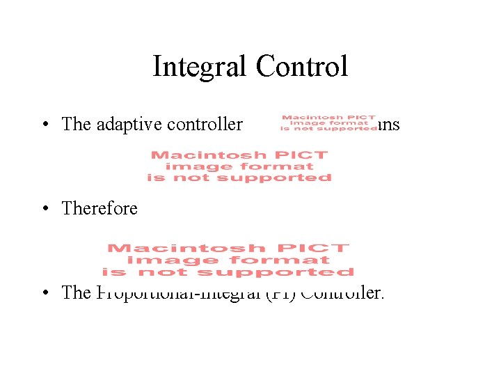
Integral Control • The adaptive controller means • Therefore • The Proportional-Integral (PI) Controller.

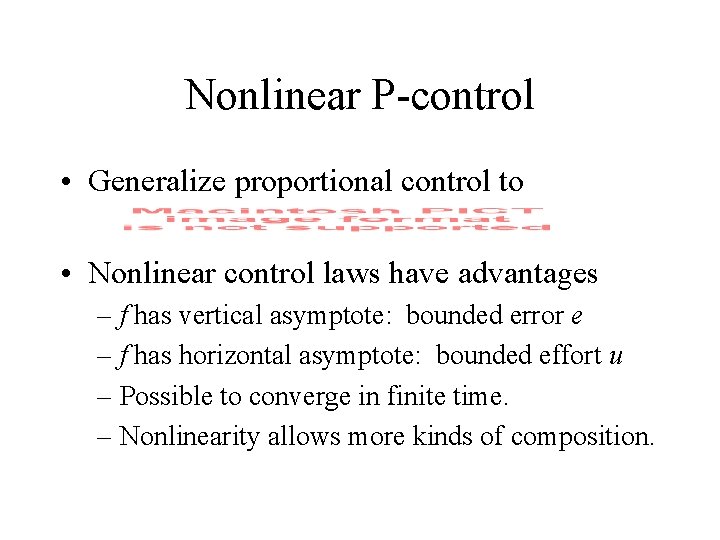
Nonlinear P-control • Generalize proportional control to • Nonlinear control laws have advantages – f has vertical asymptote: bounded error e – f has horizontal asymptote: bounded effort u – Possible to converge in finite time. – Nonlinearity allows more kinds of composition.

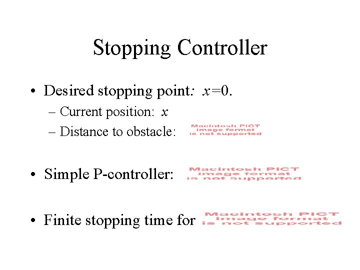
Stopping Controller • Desired stopping point: x=0. – Current position: x – Distance to obstacle: • Simple P-controller: • Finite stopping time for

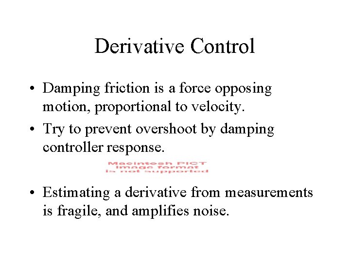
Derivative Control • Damping friction is a force opposing motion, proportional to velocity. • Try to prevent overshoot by damping controller response. • Estimating a derivative from measurements is fragile, and amplifies noise.

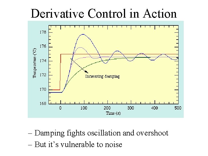
Derivative Control in Action – Damping fights oscillation and overshoot – But it’s vulnerable to noise

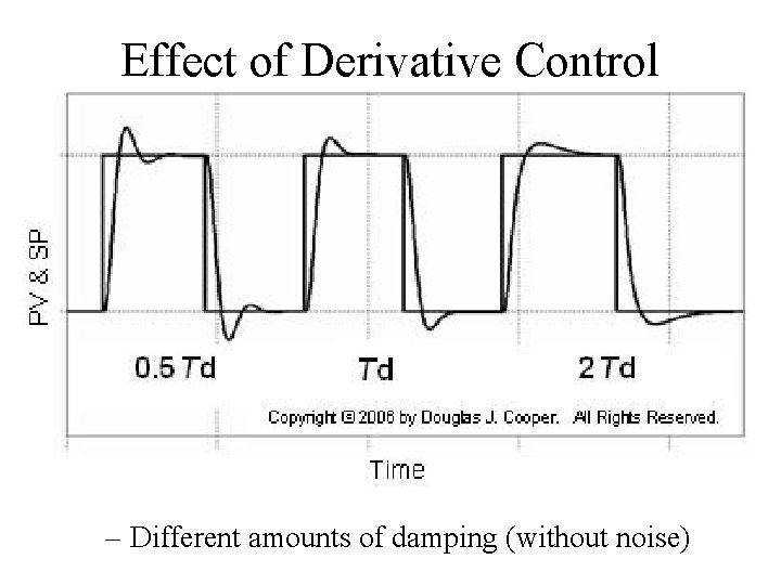
Effect of Derivative Control – Different amounts of damping (without noise)

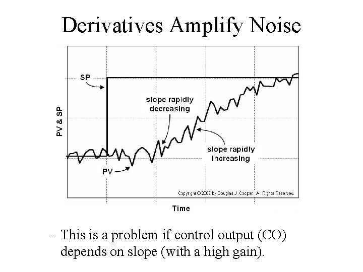
Derivatives Amplify Noise – This is a problem if control output (CO) depends on slope (with a high gain).

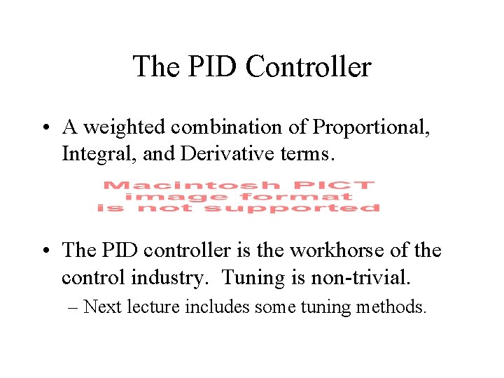
The PID Controller • A weighted combination of Proportional, Integral, and Derivative terms. • The PID controller is the workhorse of the control industry. Tuning is non-trivial. – Next lecture includes some tuning methods.

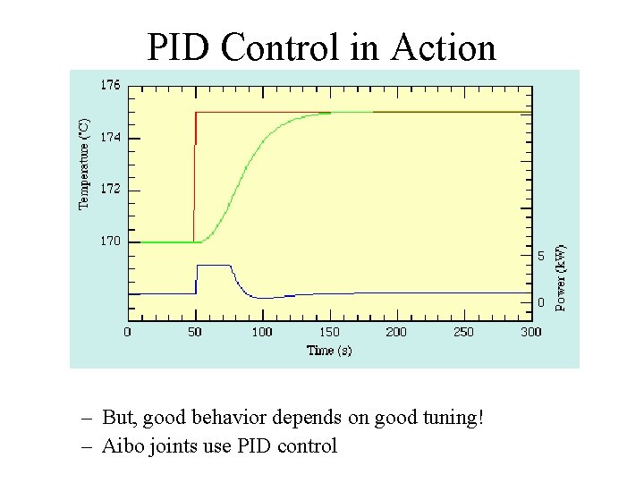
PID Control in Action – But, good behavior depends on good tuning! – Aibo joints use PID control

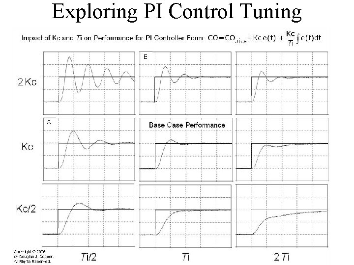
Exploring PI Control Tuning

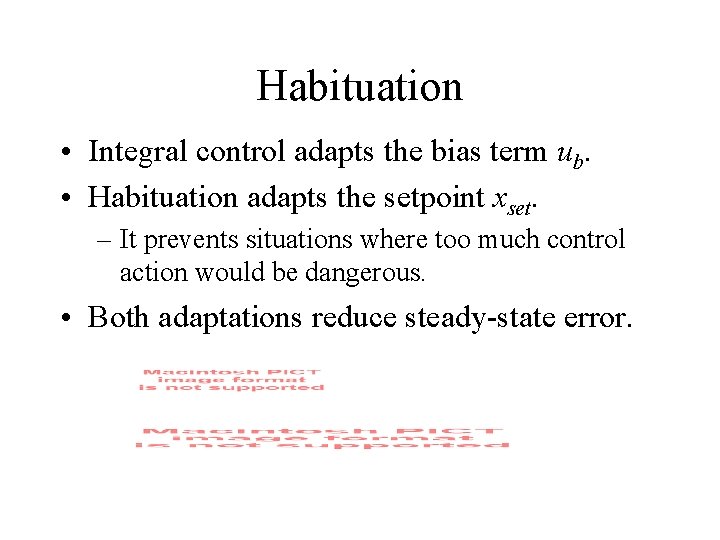
Habituation • Integral control adapts the bias term ub. • Habituation adapts the setpoint xset. – It prevents situations where too much control action would be dangerous. • Both adaptations reduce steady-state error.

Types of Controllers • Open-loop control – No sensing • Feedback control (closed-loop) – Sense error, determine control response. • Feedforward control (closed-loop) – Sense disturbance, predict resulting error, respond to predicted error before it happens. • Model-predictive control (closed-loop) – Plan trajectory to reach goal. – Take first step. – Repeat. Design open and closed-loop controllers for me to get out of the room.

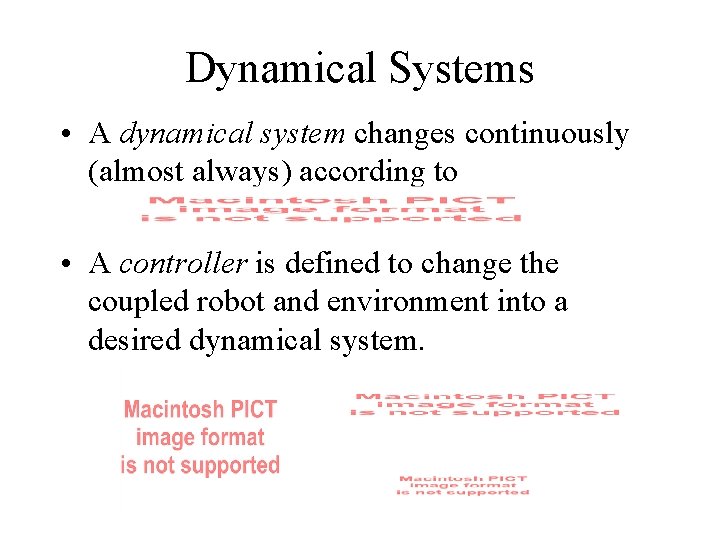
Dynamical Systems • A dynamical system changes continuously (almost always) according to • A controller is defined to change the coupled robot and environment into a desired dynamical system.

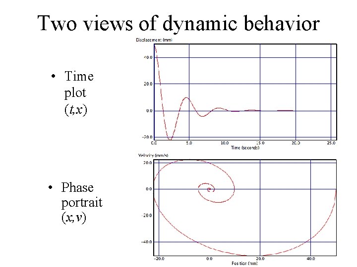
Two views of dynamic behavior • Time plot (t, x) • Phase portrait (x, v)

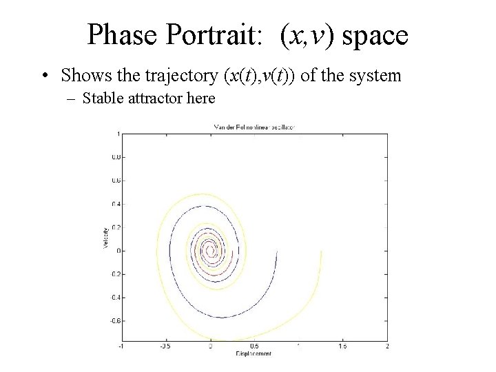
Phase Portrait: (x, v) space • Shows the trajectory (x(t), v(t)) of the system – Stable attractor here

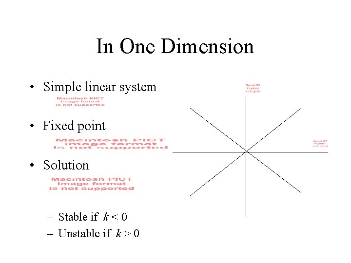
In One Dimension • Simple linear system • Fixed point • Solution – Stable if k < 0 – Unstable if k > 0

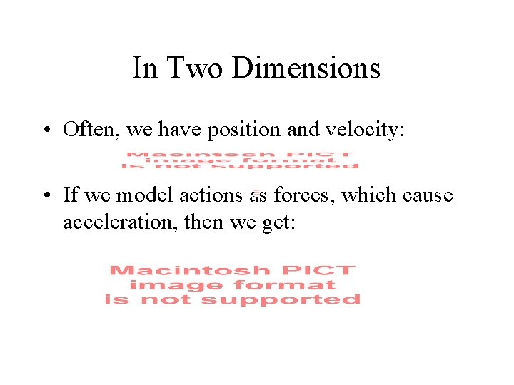
In Two Dimensions • Often, we have position and velocity: • If we model actions as forces, which cause acceleration, then we get:

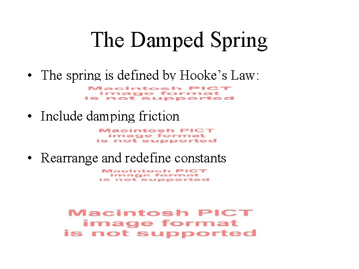
The Damped Spring • The spring is defined by Hooke’s Law: • Include damping friction • Rearrange and redefine constants

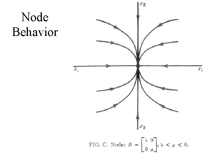
Node Behavior

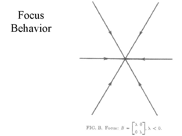
Focus Behavior

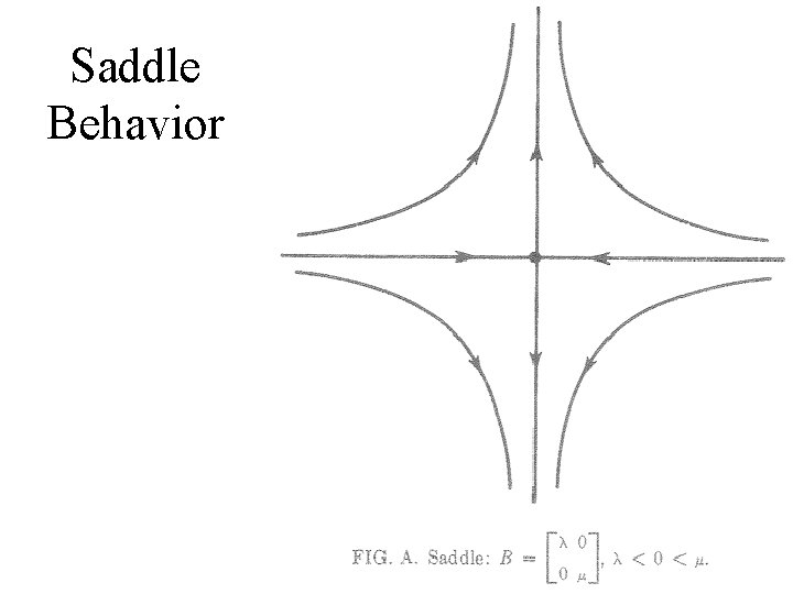
Saddle Behavior

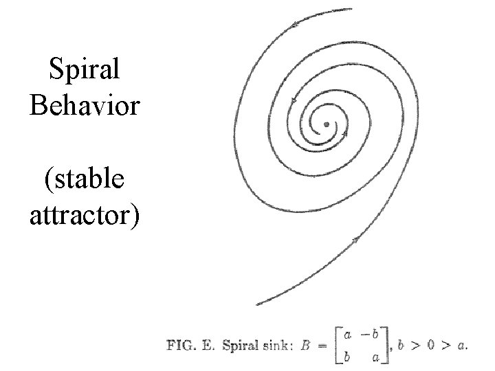
Spiral Behavior (stable attractor)

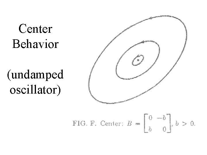
Center Behavior (undamped oscillator)

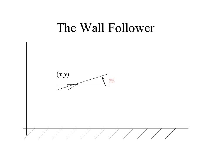
The Wall Follower (x, y)

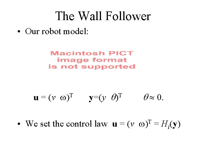
The Wall Follower • Our robot model: u = (v )T y=(y )T 0. • We set the control law u = (v )T = Hi(y)

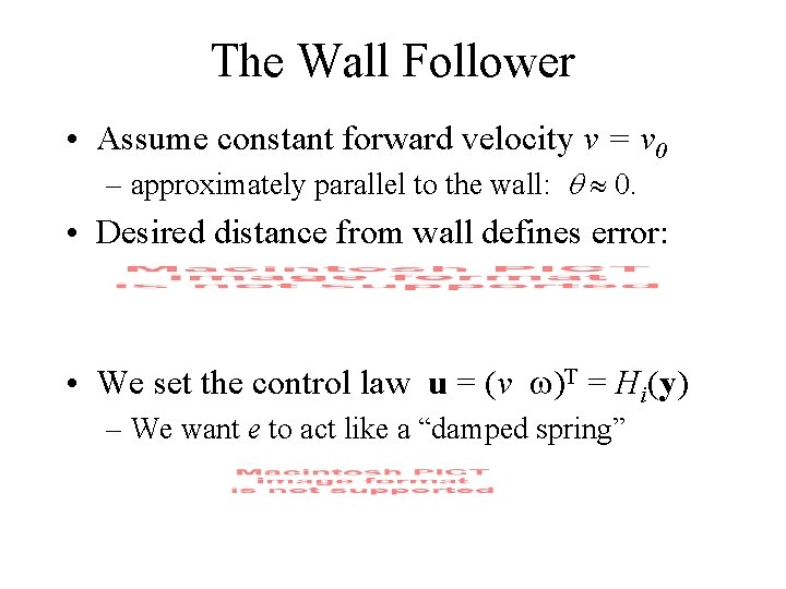
The Wall Follower • Assume constant forward velocity v = v 0 – approximately parallel to the wall: 0. • Desired distance from wall defines error: • We set the control law u = (v )T = Hi(y) – We want e to act like a “damped spring”

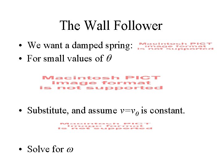
The Wall Follower • We want a damped spring: • For small values of • Substitute, and assume v=v 0 is constant. • Solve for

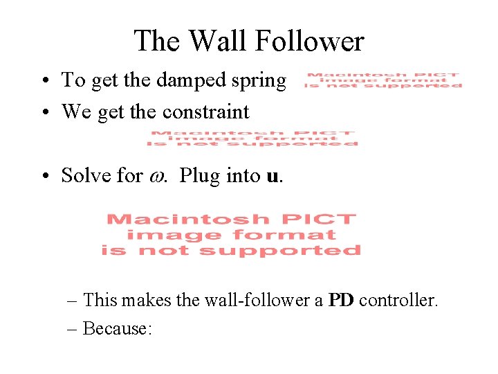
The Wall Follower • To get the damped spring • We get the constraint • Solve for . Plug into u. – This makes the wall-follower a PD controller. – Because:

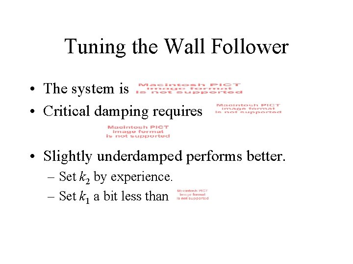
Tuning the Wall Follower • The system is • Critical damping requires • Slightly underdamped performs better. – Set k 2 by experience. – Set k 1 a bit less than

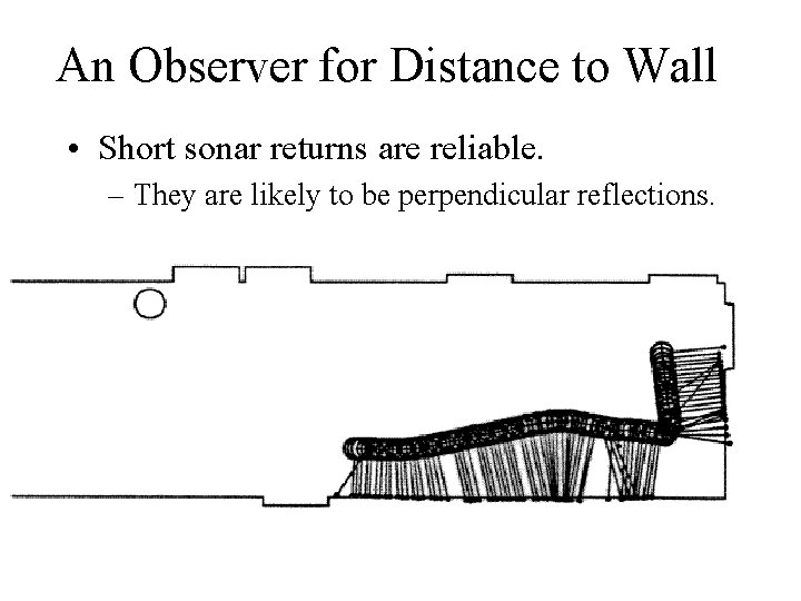
An Observer for Distance to Wall • Short sonar returns are reliable. – They are likely to be perpendicular reflections.

Alternatives • The wall follower is a PD control law. • A target seeker should probably be a PI control law, to adapt to motion. • Can try different tuning values for parameters. – This is a simple model. – Unmodeled effects might be significant.

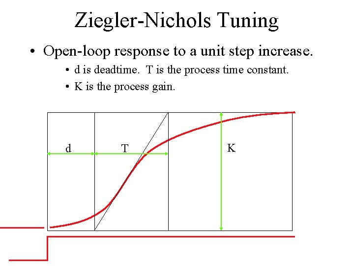
Ziegler-Nichols Tuning • Open-loop response to a unit step increase. • d is deadtime. T is the process time constant. • K is the process gain. d T K

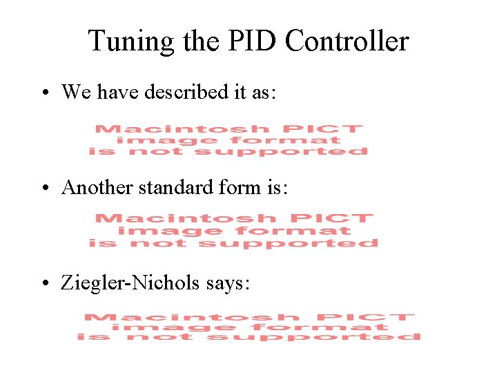
Tuning the PID Controller • We have described it as: • Another standard form is: • Ziegler-Nichols says:

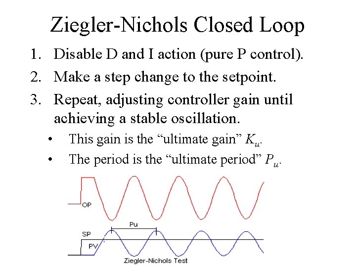
Ziegler-Nichols Closed Loop 1. Disable D and I action (pure P control). 2. Make a step change to the setpoint. 3. Repeat, adjusting controller gain until achieving a stable oscillation. • • This gain is the “ultimate gain” Ku. The period is the “ultimate period” Pu.

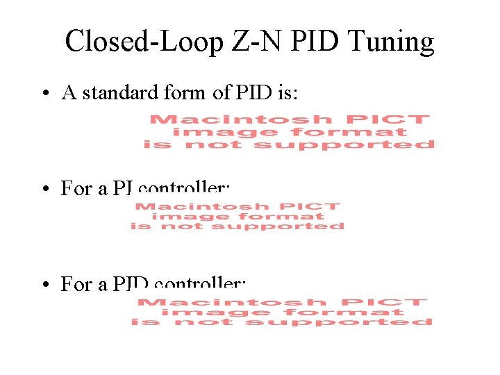
Closed-Loop Z-N PID Tuning • A standard form of PID is: • For a PI controller: • For a PID controller:

Summary of Concepts • Dynamical systems and phase portraits • Qualitative types of behavior – Stable vs unstable; nodal vs saddle vs spiral – Boundary values of parameters • Designing the wall-following control law • Tuning the PI, PD, or PID controller – Ziegler-Nichols tuning rules – For more, Google: controller tuning

Followers • A follower is a control law where the robot moves forward while keeping some error term small. – Open-space follower – Wall follower – Coastal navigator – Color follower

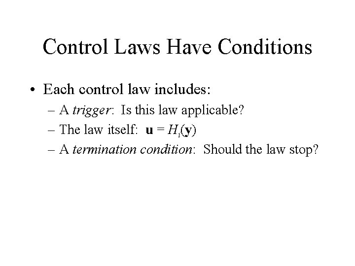
Control Laws Have Conditions • Each control law includes: – A trigger: Is this law applicable? – The law itself: u = Hi(y) – A termination condition: Should the law stop?

Open-Space Follower • Move in the direction of large amounts of open space. • Wiggle as needed to avoid specular reflections. • Turn away from obstacles. • Turn or back out of blind alleys.

Wall Follower • • Detect and follow right or left wall. PD control law. Tune to avoid large oscillations. Terminate on obstacle or wall vanishing.

Coastal Navigator • Join wall-followers to follow a complex “coastline” • When a wall-follower terminates, make the appropriate turn, detect a new wall, and continue. • Inside and outside corners, 90 and 180 deg. • Orbit a box, a simple room, or the desks.

Color Follower • Move to keep a desired color centered in the camera image. • Train a color region from a given image. • Follow an orange ball on a string, or a brightly-colored T-shirt.

Problems and Solutions • • Time delay Static friction Pulse-width modulation Integrator wind-up Chattering Saturation, dead-zones, backlash Parameter drift

Unmodeled Effects • Every controller depends on its simplified model of the world. – Every model omits almost everything. • If unmodeled effects become significant, the controller’s model is wrong, – so its actions could be seriously wrong. • Most controllers need special case checks. – Sometimes it needs a more sophisticated model.

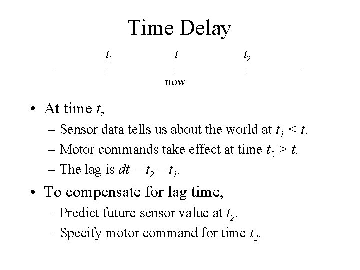
Time Delay t 1 t t 2 now • At time t, – Sensor data tells us about the world at t 1 < t. – Motor commands take effect at time t 2 > t. – The lag is dt = t 2 t 1. • To compensate for lag time, – Predict future sensor value at t 2. – Specify motor command for time t 2.

Predicting Future Sensor Values • Later, observers will help us make better predictions. • Now, use a simple prediction method: – If sensor s is changing at rate ds/dt, – At time t, we get s(t 1), where t 1 < t, – Estimate s(t 2) = s(t 1) + ds/dt * (t 2 - t 1). • Use s(t 2) to determine motor signal u(t) that will take effect at t 2.

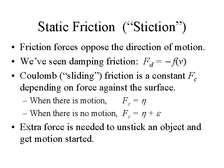
Static Friction (“Stiction”) • Friction forces oppose the direction of motion. • We’ve seen damping friction: Fd = f(v) • Coulomb (“sliding”) friction is a constant Fc depending on force against the surface. – When there is motion, Fc = – When there is no motion, Fc = + • Extra force is needed to unstick an object and get motion started.

Why is Stiction Bad? • Non-zero steady-state error. • Stalled motors draw high current. – Running motor converts current to motion. – Stalled motor converts more current to heat. • Whining from pulse-width modulation. – Mechanical parts bending at pulse frequency.

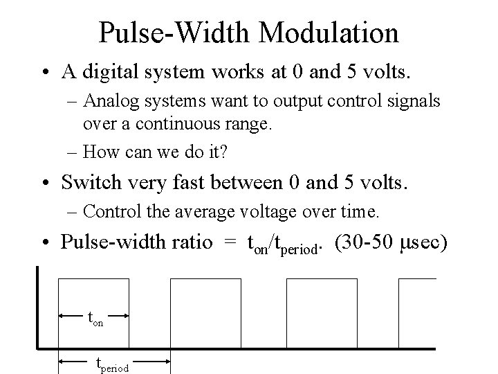
Pulse-Width Modulation • A digital system works at 0 and 5 volts. – Analog systems want to output control signals over a continuous range. – How can we do it? • Switch very fast between 0 and 5 volts. – Control the average voltage over time. • Pulse-width ratio = ton/tperiod. (30 -50 sec) ton tperiod

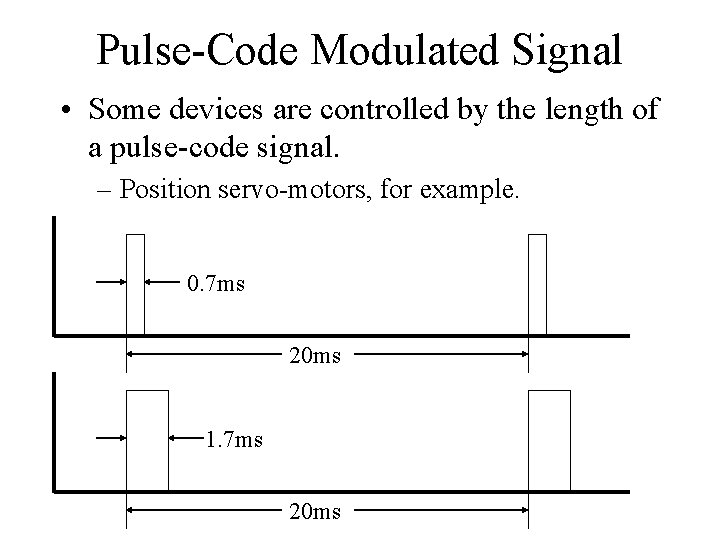
Pulse-Code Modulated Signal • Some devices are controlled by the length of a pulse-code signal. – Position servo-motors, for example. 0. 7 ms 20 ms 1. 7 ms 20 ms

Integrator Wind-Up • Suppose we have a PI controller • Motion might be blocked, but the integral is winding up more and more control action. • Reset the integrator on significant events.

Chattering • Changing modes rapidly and continually. – Bang-Bang controller with thresholds set too close to each other. – Integrator wind-up due to stiction near the setpoint, causing jerk, overshoot, and repeat.

Dead Zone • A region where controller output does not affect the state of the system. – A system caught by static friction. – Cart-pole system when the pendulum is horizontal. – Cruise control when the car is stopped. • Integral control and dead zones can combine to cause integrator wind-up problems.

Saturation • Control actions cannot grow indefinitely. – There is a maximum possible output. – Physical systems are necessarily nonlinear. • It might be nice to have bounded error by having infinite response. – But it doesn’t happen in the real world.

Backlash • Real gears are not perfect connections. – There is space between the teeth. • On reversing direction, there is a short time when the input gear is turning, but the output gear is not.

Parameter Drift • Hidden parameters can change the behavior of the robot, for no obvious reason. – Performance depends on battery voltage. – Repeated discharge/charge cycles age the battery. • A controller may compensate for small parameter drift until it passes a threshold. – Then a problem suddenly appears. – Controlled systems make problems harder to find

Unmodeled Effects • Every controller depends on its simplified model of the world. – Every model omits almost everything. • If unmodeled effects become significant, the controller’s model is wrong, – so its actions could be seriously wrong. • Most controllers need special case checks. – Sometimes it needs a more sophisticated model.