Basic Business Statistics 10 th Edition Chapter 4

Learning Objectives In this chapter, you learn: n n Basic probability concepts and definitions Conditional probability To use Bayes’ Theorem to revise probabilities Various counting rules Basic Business Statistics, 10 e © 2006 Prentice-Hall, Inc. 2

Important Terms n n Probability – the chance that an uncertain event will occur (always between 0 and 1) Event – Each possible outcome of a variable Simple Event – an event that can be described by a single characteristic Sample Space – the collection of all possible events Basic Business Statistics, 10 e © 2006 Prentice-Hall, Inc. 3

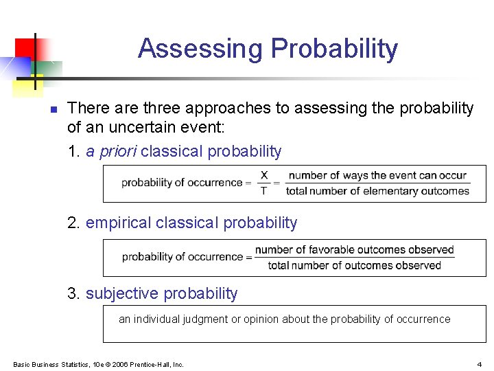
Assessing Probability n There are three approaches to assessing the probability of an uncertain event: 1. a priori classical probability 2. empirical classical probability 3. subjective probability an individual judgment or opinion about the probability of occurrence Basic Business Statistics, 10 e © 2006 Prentice-Hall, Inc. 4

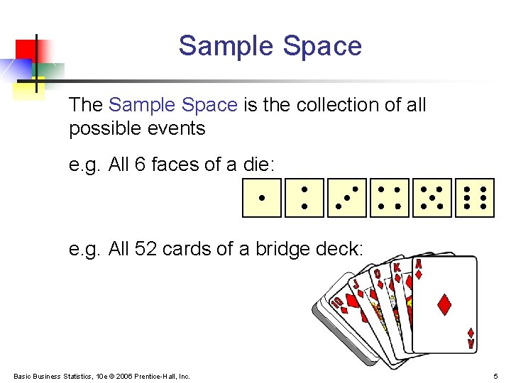
Sample Space The Sample Space is the collection of all possible events e. g.

Events n Simple event n n n Complement of an event A (denoted A’) n n n An outcome from a sample space with one characteristic e. g. , A red card from a deck of cards All outcomes that are not part of event A e. g. , All cards that are not diamonds Joint event n n Involves two or more characteristics simultaneously e. g. , An ace that is also red from a deck of cards Basic Business Statistics, 10 e © 2006 Prentice-Hall, Inc. 6

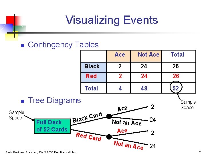
Visualizing Events n Contingency Tables Ace n Sample Space 2 24 26 Red 2 24 26 Total 4 48 52 ard C k lac B Red C Basic Business Statistics, 10 e © 2006 Prentice-Hall, Inc. Total Black Tree Diagrams Full Deck of 52 Cards Not Ace ard 2 Ace Not an Sample Space 24 2 Ace 24 7

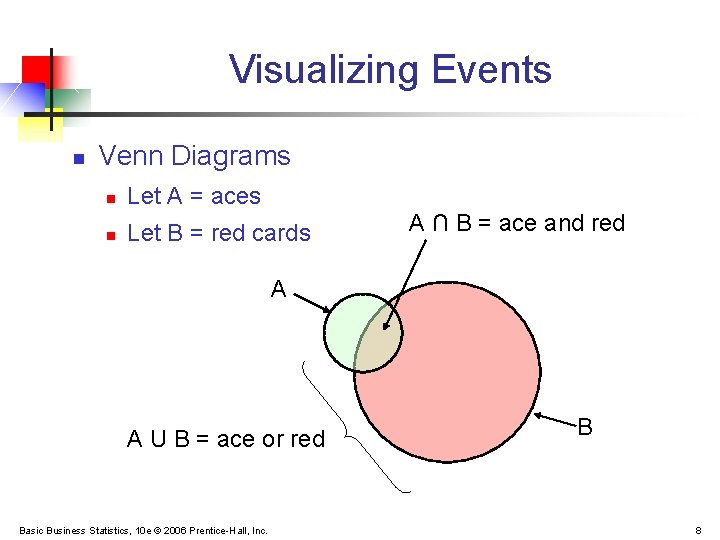
Visualizing Events n Venn Diagrams n Let A = aces n Let B =

Mutually Exclusive Events n Mutually exclusive events n Events that cannot occur together example: A = queen of diamonds; B = queen of clubs n Events A and B are mutually exclusive Basic Business Statistics, 10 e © 2006 Prentice-Hall, Inc. 9

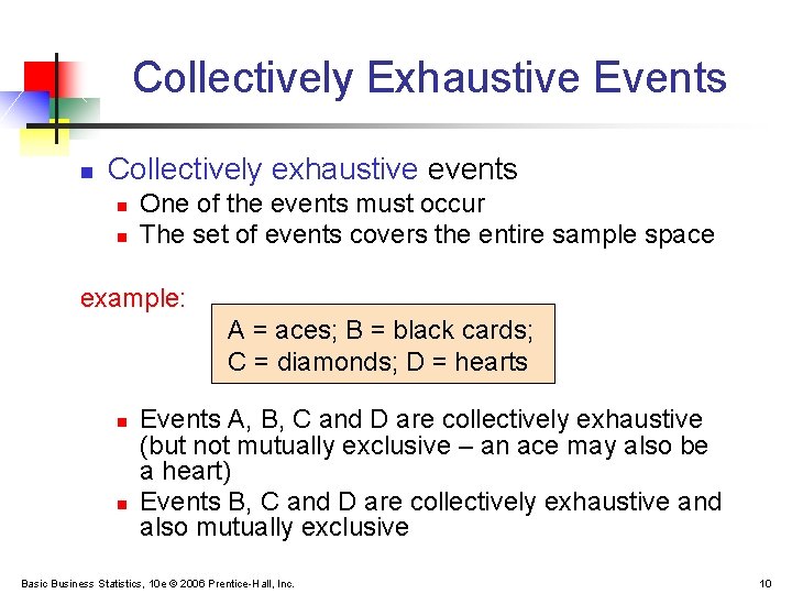
Collectively Exhaustive Events n Collectively exhaustive events n n One of the events must occur The set of events covers the entire sample space example: A = aces; B = black cards; C = diamonds; D = hearts n n Events A, B, C and D are collectively exhaustive (but not mutually exclusive – an ace may also be a heart) Events B, C and D are collectively exhaustive and also mutually exclusive Basic Business Statistics, 10 e © 2006 Prentice-Hall, Inc. 10

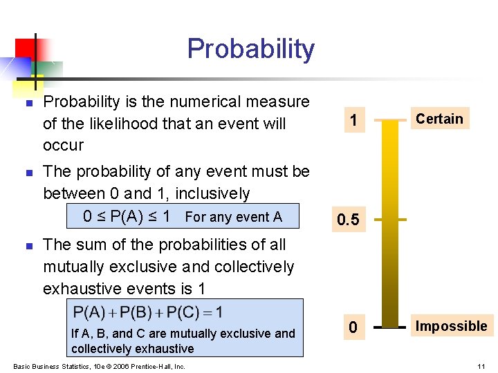
Probability n n n Probability is the numerical measure of the likelihood that an event will occur The probability of any event must be between 0 and 1, inclusively 0 ≤ P(A) ≤ 1 For any event A 1 Certain 0. 5 The sum of the probabilities of all mutually exclusive and collectively exhaustive events is 1 If A, B, and C are mutually exclusive and collectively exhaustive Basic Business Statistics, 10 e © 2006 Prentice-Hall, Inc. 0 Impossible 11

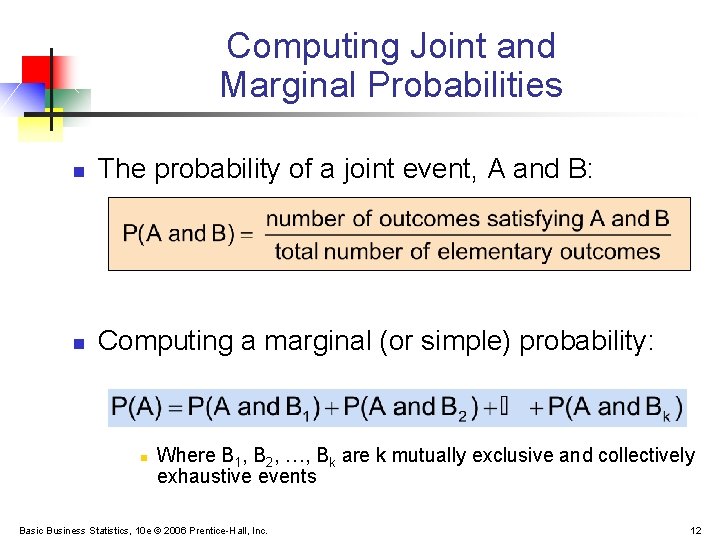
Computing Joint and Marginal Probabilities n The probability of a joint event, A and B: n Computing a marginal (or simple) probability: n Where B 1, B 2, …, Bk are k mutually exclusive and collectively exhaustive events Basic Business Statistics, 10 e © 2006 Prentice-Hall, Inc. 12

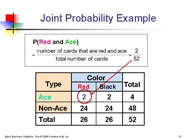
Joint Probability Example P(Red and Ace) Type Color Red Black Total Ace 2 2

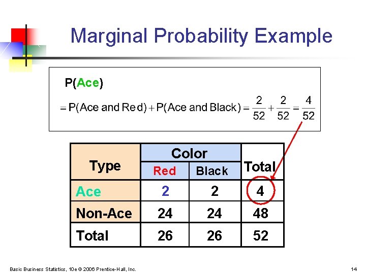
Marginal Probability Example P(Ace) Type Color Red Black Total Ace 2 2 4 Non-Ace

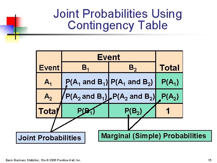
Joint Probabilities Using Contingency Table Event B 1 Event B 2 Total A 1 P(A 1 and B 1) P(A 1 and B 2) A 2 P(A 2 and B 1) P(A 2 and B 2) P(A 2) Total P(B 1) Joint Probabilities Basic Business Statistics, 10 e © 2006 Prentice-Hall, Inc. P(B 2) P(A 1) 1 Marginal (Simple) Probabilities 15

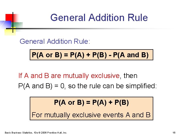
General Addition Rule: P(A or B) = P(A) + P(B) - P(A and B) If A and B are mutually exclusive, then P(A and B) = 0, so the rule can be simplified: P(A or B) = P(A) + P(B) For mutually exclusive events A and B Basic Business Statistics, 10 e © 2006 Prentice-Hall, Inc. 16

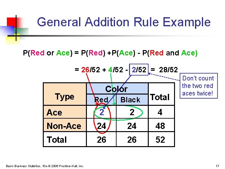
General Addition Rule Example P(Red or Ace) = P(Red) +P(Ace) - P(Red and Ace) = 26/52 + 4/52 - 2/52 = 28/52 Type Color Red Black Total Ace 2 2 4 Non-Ace 24 24 48 Total 26 26 52 Basic Business Statistics, 10 e © 2006 Prentice-Hall, Inc. Don’t count the two red aces twice! 17

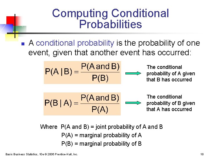
Computing Conditional Probabilities n A conditional probability is the probability of one event, given that another event has occurred: The conditional probability of A given that B has occurred The conditional probability of B given that A has occurred Where P(A and B) = joint probability of A and B P(A) = marginal probability of A P(B) = marginal probability of B Basic Business Statistics, 10 e © 2006 Prentice-Hall, Inc. 18

Conditional Probability Example n n Of the cars on a used car lot, 70% have air conditioning (AC) and 40% have a CD player (CD). 20% of the cars have both. What is the probability that a car has a CD player, given that it has AC ? i. e. , we want to find P(CD | AC) Basic Business Statistics, 10 e © 2006 Prentice-Hall, Inc. 19

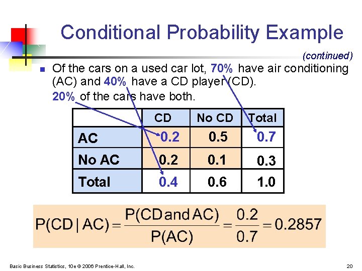
Conditional Probability Example (continued) n Of the cars on a used car lot, 70% have air conditioning (AC) and 40% have a CD player (CD). 20% of the cars have both. CD No CD Total AC 0. 2 0. 5 0. 7 No AC 0. 2 0. 1 0. 3 Total 0. 4 0. 6 1. 0 Basic Business Statistics, 10 e © 2006 Prentice-Hall, Inc. 20

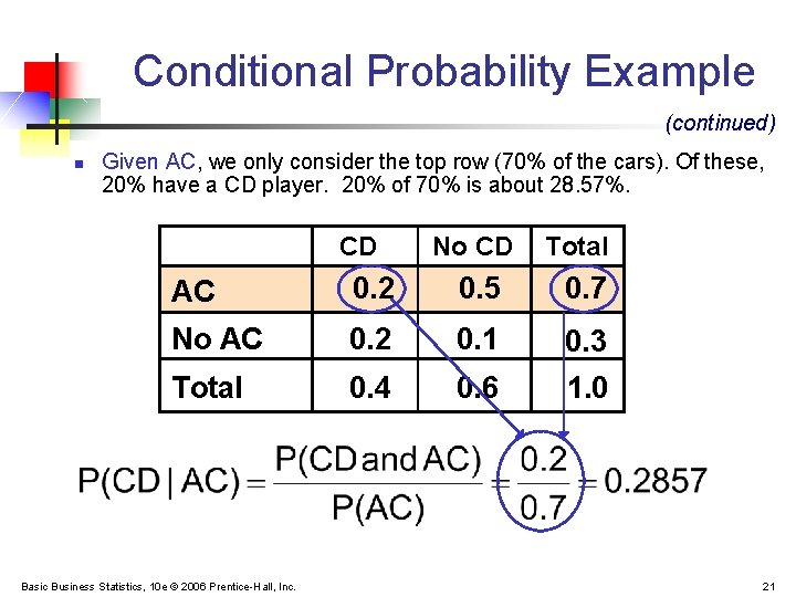
Conditional Probability Example (continued) n Given AC, we only consider the top row (70% of the cars). Of these, 20% have a CD player. 20% of 70% is about 28. 57%. CD No CD Total AC 0. 2 0. 5 0. 7 No AC 0. 2 0. 1 0. 3 Total 0. 4 0. 6 1. 0 Basic Business Statistics, 10 e © 2006 Prentice-Hall, Inc. 21

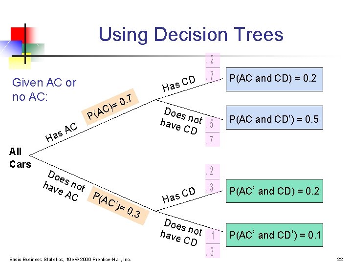
Using Decision Trees D as C Given AC or no AC: . 7 0 = ) C P(A C A as H All Cars Doe hav s not e. A P(A C C’) =0. 3 Basic Business Statistics, 10 e © 2006 Prentice-Hall, Inc. H Doe s have not CD D C Has Doe s have not CD P(AC and CD) = 0. 2 P(AC and CD’) = 0. 5 P(AC’ and CD) = 0. 2 P(AC’ and CD’) = 0. 1 22

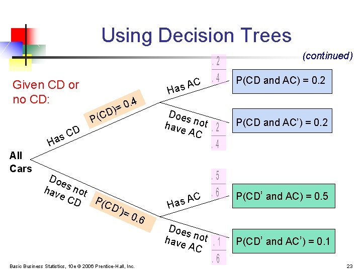
Using Decision Trees (continued) C as A Given CD or no CD: D 0 D)= . 4 P(C C as H All Cars Doe hav s not e. C D P(C D’) =0. 6 Basic Business Statistics, 10 e © 2006 Prentice-Hall, Inc. H Doe s have not AC C A Has Doe s have not AC P(CD and AC) = 0. 2 P(CD and AC’) = 0. 2 P(CD’ and AC) = 0. 5 P(CD’ and AC’) = 0. 1 23

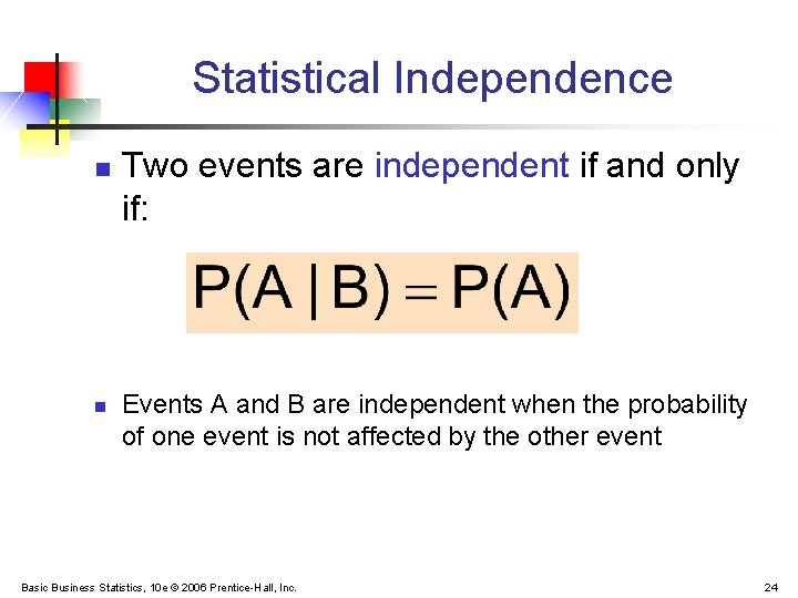
Statistical Independence n n Two events are independent if and only if: Events A and B are independent when the probability of one event is not affected by the other event Basic Business Statistics, 10 e © 2006 Prentice-Hall, Inc. 24

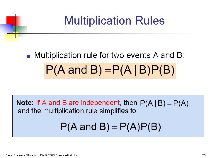
Multiplication Rules n Multiplication rule for two events A and B: Note: If A and B are independent, then and the multiplication rule simplifies to Basic Business Statistics, 10 e © 2006 Prentice-Hall, Inc. 25

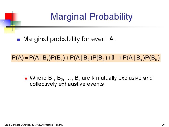
Marginal Probability n Marginal probability for event A: n Where B 1, B 2, …, Bk are k mutually exclusive and collectively exhaustive events Basic Business Statistics, 10 e © 2006 Prentice-Hall, Inc. 26

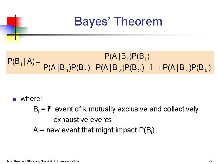
Bayes’ Theorem n where: Bi = ith event of k mutually exclusive and collectively

Bayes’ Theorem Example n n n A drilling company has estimated a 40% chance of striking oil for their new well. A detailed test has been scheduled for more information. Historically, 60% of successful wells have had detailed tests, and 20% of unsuccessful wells have had detailed tests. Given that this well has been scheduled for a detailed test, what is the probability that the well will be successful? Basic Business Statistics, 10 e © 2006 Prentice-Hall, Inc. 28

Bayes’ Theorem Example (continued) n Let S = successful well U = unsuccessful well n P(S) = 0. 4 , P(U) = 0. 6 n Define the detailed test event as D n Conditional probabilities: P(D|S) = 0. 6 n (prior probabilities) P(D|U) = 0. 2 Goal is to find P(S|D) Basic Business Statistics, 10 e © 2006 Prentice-Hall, Inc. 29

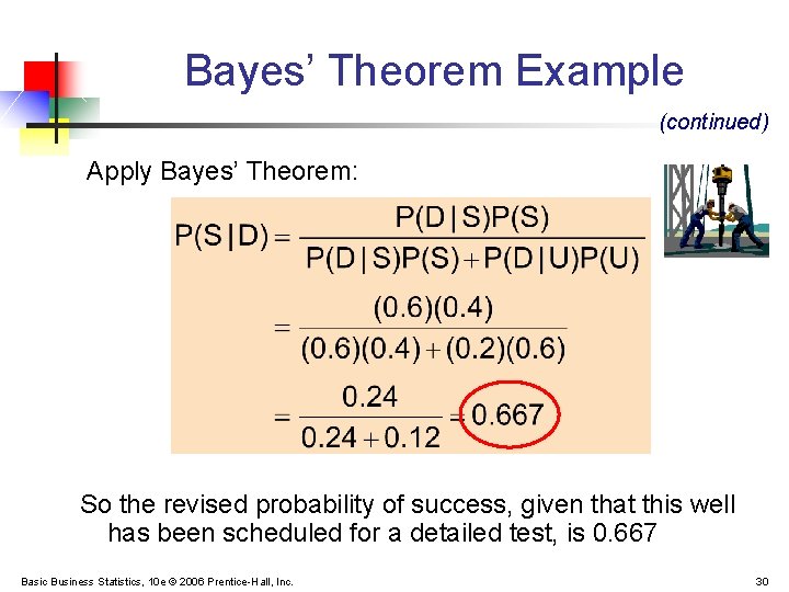
Bayes’ Theorem Example (continued) Apply Bayes’ Theorem: So the revised probability of success, given that this well has been scheduled for a detailed test, is 0. 667 Basic Business Statistics, 10 e © 2006 Prentice-Hall, Inc. 30

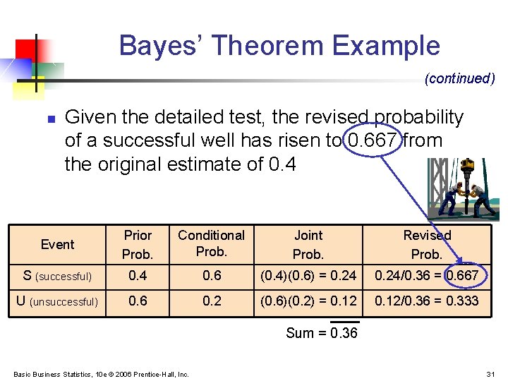
Bayes’ Theorem Example (continued) n Given the detailed test, the revised probability of a successful well has risen to 0. 667 from the original estimate of 0. 4 Event Prior Prob. Conditional Prob. Joint Prob. Revised Prob. S (successful) 0. 4 0. 6 (0. 4)(0. 6) = 0. 24/0. 36 = 0. 667 U (unsuccessful) 0. 6 0. 2 (0. 6)(0. 2) = 0. 12/0. 36 = 0. 333 Sum = 0. 36 Basic Business Statistics, 10 e © 2006 Prentice-Hall, Inc. 31

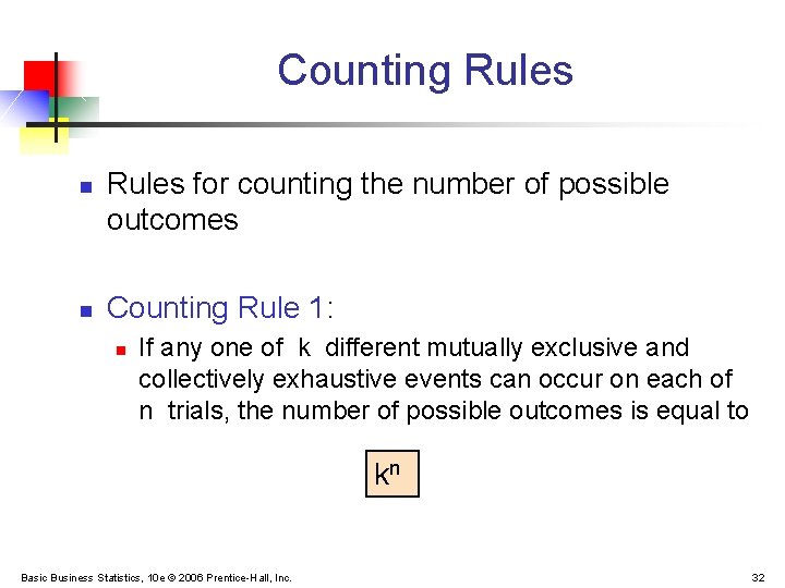
Counting Rules n n Rules for counting the number of possible outcomes Counting Rule 1: n If any one of k different mutually exclusive and collectively exhaustive events can occur on each of n trials, the number of possible outcomes is equal to kn Basic Business Statistics, 10 e © 2006 Prentice-Hall, Inc. 32

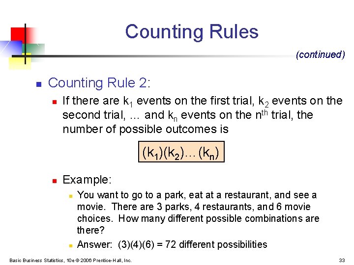
Counting Rules (continued) n Counting Rule 2: n If there are k 1 events on the first trial, k 2 events on the second trial, … and kn events on the nth trial, the number of possible outcomes is (k 1)(k 2)…(kn) n Example: n n You want to go to a park, eat at a restaurant, and see a movie. There are 3 parks, 4 restaurants, and 6 movie choices. How many different possible combinations are there? Answer: (3)(4)(6) = 72 different possibilities Basic Business Statistics, 10 e © 2006 Prentice-Hall, Inc. 33

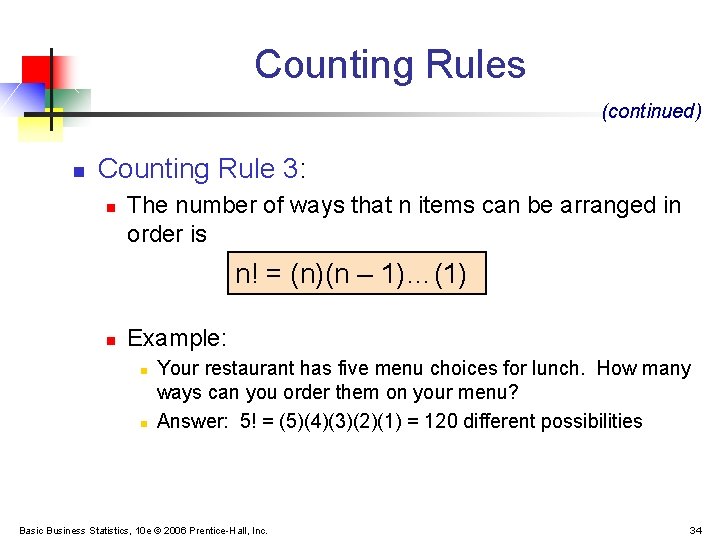
Counting Rules (continued) n Counting Rule 3: n The number of ways that n items can be arranged in order is n! = (n)(n – 1)…(1) n Example: n n Your restaurant has five menu choices for lunch. How many ways can you order them on your menu? Answer: 5! = (5)(4)(3)(2)(1) = 120 different possibilities Basic Business Statistics, 10 e © 2006 Prentice-Hall, Inc. 34

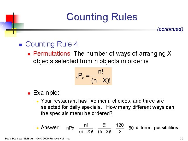
Counting Rules (continued) n Counting Rule 4: n n Permutations: The number of ways of arranging X objects selected from n objects in order is Example: n n Your restaurant has five menu choices, and three are selected for daily specials. How many different ways can the specials menu be ordered? Answer: Basic Business Statistics, 10 e © 2006 Prentice-Hall, Inc. different possibilities 35

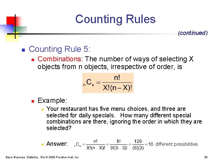
Counting Rules (continued) n Counting Rule 5: n n Combinations: The number of ways of selecting X objects from n objects, irrespective of order, is Example: n n Your restaurant has five menu choices, and three are selected for daily specials. How many different special combinations are there, ignoring the order in which they are selected? Answer: Basic Business Statistics, 10 e © 2006 Prentice-Hall, Inc. different possibilities 36

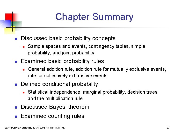
Chapter Summary n Discussed basic probability concepts n n Examined basic probability rules n n Sample spaces and events, contingency tables, simple probability, and joint probability General addition rule, addition rule for mutually exclusive events, rule for collectively exhaustive events Defined conditional probability n Statistical independence, marginal probability, decision trees, and the multiplication rule n Discussed Bayes’ theorem n Examined counting rules Basic Business Statistics, 10 e © 2006 Prentice-Hall, Inc. 37