BALTIMORE METROPOLITAN COUNCIL MODEL ENHANCEMENTS FOR THE RED

BALTIMORE METROPOLITAN COUNCIL MODEL ENHANCEMENTS FOR THE RED LINE PROJECT • • • AMPO TRAVEL MODEL WORK GROUP March 20, 2006

BMC Enhanced Model–Background • Update to the Baltimore region travel demand model • MTA provided funding • Developed by William G. Allen with assistance from BMC staff • Motivation/Goal • Revised mode choice model to meet FTA technical analysis of user benefits utilizing SUMMIT • Analysis of proposed Red Line to request New Starts funding • Develop one regional model used for long/short range regional planning, regional conformity analysis, and FTA new starts analysis

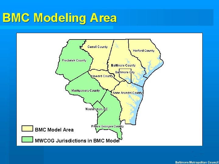
BMC Modeling Area BMC Model Area MWCOG Jurisdictions in BMC Model

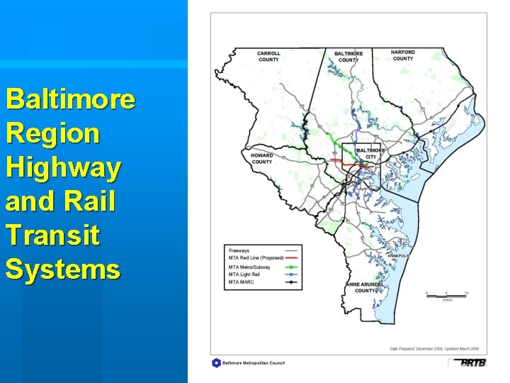
Baltimore Region Highway and Rail Transit Systems

BMC Enhanced Model–Objectives • • • User friendly – logical input file names Reduce off-model data preparation Reduce number of input files Incorporation of 2001 NHTS data Meet Requirements of FTA • Remove “cliff” functions • Use same coefficients for transit and auto time • Eliminate geographic bias constants • Produce input files for SUMMIT

BMC Enhanced Model–Status • • • Draft functioning model as of February 2006 Conducting sensitivity test designed to evaluate estimated changes in demand BMC staff developing a further understanding of the model through application, documentation, and development of user guide/local training session Extensive quality control checking of all model aspects Model runs in 9 to 10 hours (previous model 6 to 7 hours)

Trip Generation Features • Demographic models • Households by size (5)/income (4) • • Urban Size (Baltimore City, DC, Montgomery, PG) Suburban Size (All Others) Urban Income (Baltimore City and DC) Suburban Income (All Others) • Workers (4)/income (4) • Workers for Washington region must be estimated based on household size and income from PUMS • Income split is 10/15/20/55% of households (lowest to highest)

Trip Generation Features (Cont’d) • 10 trip purposes • Home-Based Work, Shop, Other, and School • Non-Home-Based JTW, JAW, and OBO • Truck CV, MTK, and HTK Nine area types based on household and employment density • Trip productions by rates for different HH size/income and worker/income combinations • Trip attractions by regression equation, adjusted by area type •

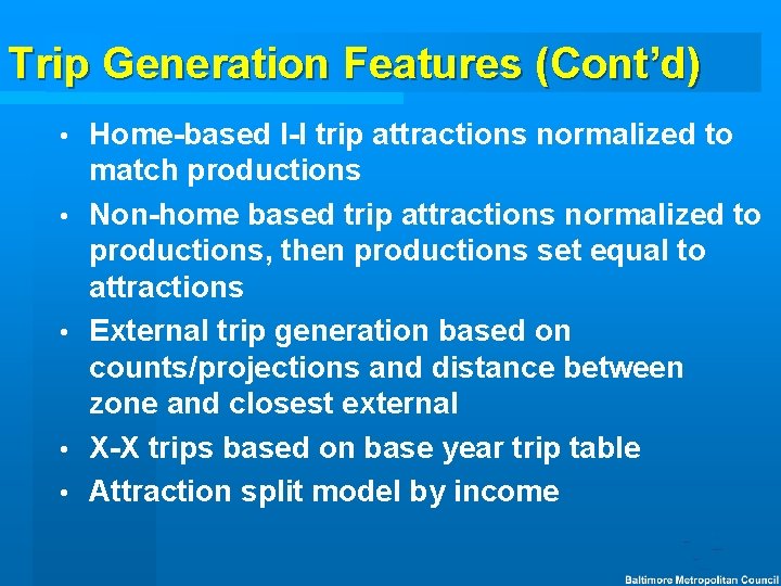
Trip Generation Features (Cont’d) • • • Home-based I-I trip attractions normalized to match productions Non-home based trip attractions normalized to productions, then productions set equal to attractions External trip generation based on counts/projections and distance between zone and closest external X-X trips based on base year trip table Attraction split model by income

2000 Density Codes

2030 Density Codes

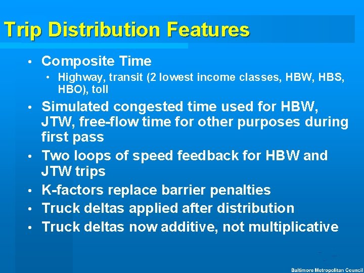
Trip Distribution Features • Composite Time • Highway, transit (2 lowest income classes, HBW, HBS, HBO), toll • • • Simulated congested time used for HBW, JTW, free-flow time for other purposes during first pass Two loops of speed feedback for HBW and JTW trips K-factors replace barrier penalties Truck deltas applied after distribution Truck deltas now additive, not multiplicative

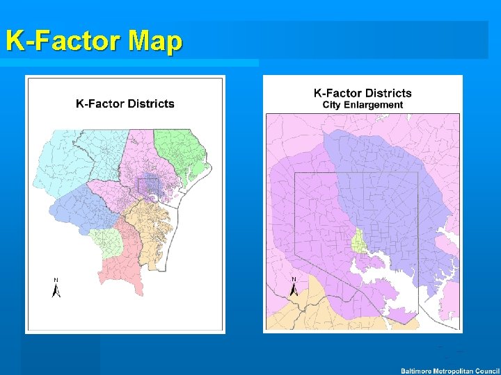
K-Factor Map

Mode Choice Features • New transit access pre-process • TP+, Arc. Info, Microsoft Access • Create up to 9 walk links per mode, unlimited drive links within 30 minutes • Create ½ mile buffer around local transit lines and express bus and rail stops • Identify walk access share of each zone within buffer • Determine average walk time for bus, rail, commuter rail, peak and off-peak • Select links from those actually used in pathbuilding limited in number and distance/time

Mode Choice Features • New nested logit mode choice model • Same structure for all non-school purposes • Model for school trips includes a top-level school bus nest Parking cost model • Three levels of auto occupancy • Three transit modes • Two access modes •

Mode Choice Features (Continued) Peak and off-peak transit networks • “Freeze-dry” Washington mode choice • Dummy links for DC transit access/egress •

Mode Choice Structure

Mode Choice Structure–School

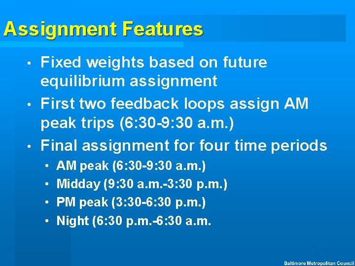
Assignment Features Fixed weights based on future equilibrium assignment • First two feedback loops assign AM peak trips (6: 30 -9: 30 a. m. ) • Final assignment for four time periods • • • AM peak (6: 30 -9: 30 a. m. ) Midday (9: 30 a. m. -3: 30 p. m. ) PM peak (3: 30 -6: 30 p. m. ) Night (6: 30 p. m. -6: 30 a. m.

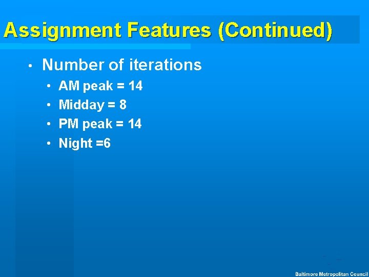
Assignment Features (Continued) • Number of iterations • • AM peak = 14 Midday = 8 PM peak = 14 Night =6

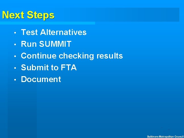
Next Steps • • • Test Alternatives Run SUMMIT Continue checking results Submit to FTA Document