Backprop Representations Garrison W Cottrell Garys Unbelievable Research

Backprop, Representations, Garrison W. Cottrell Gary's Unbelievable Research Unit (GURU) Computer Science and Engineering Department Temporal Dynamics of Learning Center Institute for Neural Computation UCSD 1

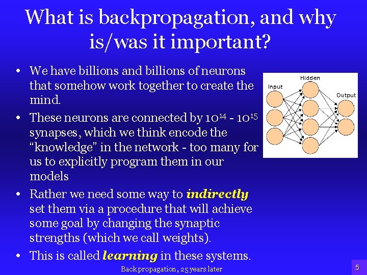
What is backpropagation, and why is/was it important? • We have billions and billions of neurons that somehow work together to create the mind. • These neurons are connected by 1014 - 1015 synapses, which we think encode the “knowledge” in the network - too many for us to explicitly program them in our models • Rather we need some way to indirectly set them via a procedure that will achieve some goal by changing the synaptic strengths (which we call weights). • This is called learning in these systems. Back propagation, 25 years later 5

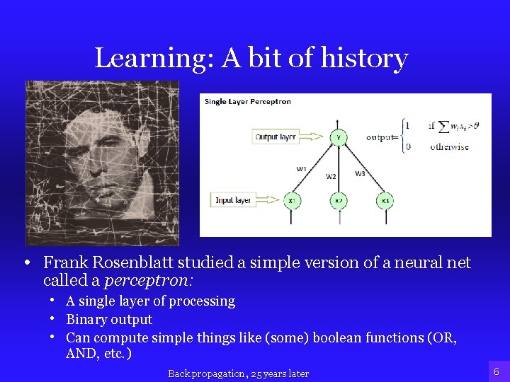
Learning: A bit of history • Frank Rosenblatt studied a simple version of a neural net called a perceptron: • A single layer of processing • Binary output • Can compute simple things like (some) boolean functions (OR, AND, etc. ) Back propagation, 25 years later 6

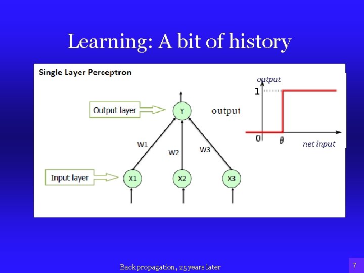
Learning: A bit of history output net input Back propagation, 25 years later 7

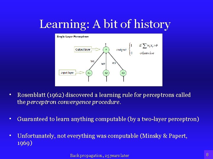
Learning: A bit of history • Rosenblatt (1962) discovered a learning rule for perceptrons called the perceptron convergence procedure. • Guaranteed to learn anything computable (by a two-layer perceptron) • Unfortunately, not everything was computable (Minsky & Papert, 1969) Back propagation, 25 years later 8

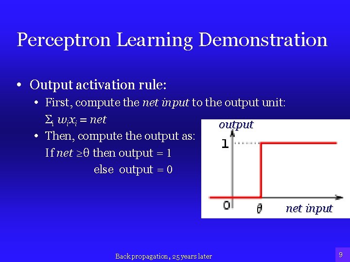
Perceptron Learning Demonstration • Output activation rule: • First, compute the net input to the output unit: Σi wixi = net • Then, compute the output as: If net ≥θ then output = 1 else output = 0 output net input Back propagation, 25 years later 9

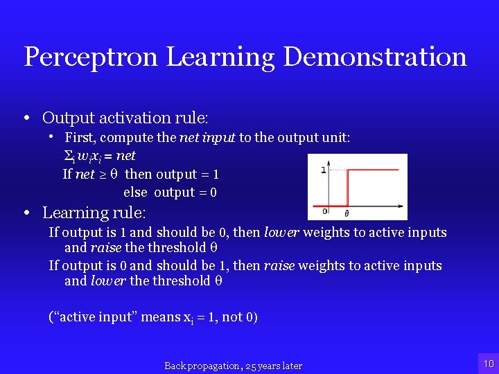
Perceptron Learning Demonstration • Output activation rule: • First, compute the net input to the output unit: Σi wixi = net If net ≥ θ then output = 1 else output = 0 • Learning rule: If output is 1 and should be 0, then lower weights to active inputs and raise threshold θ If output is 0 and should be 1, then raise weights to active inputs and lower the threshold θ (“active input” means xi = 1, not 0) Back propagation, 25 years later 10

• STOP HERE FOR DEMO Back propagation, 25 years later 11

Characteristics of perceptron learning • Supervised learning: Gave it a set of input-output examples for it to model the function (a teaching signal) • Error correction learning: only correct it when it is wrong. • Random presentation of patterns. • Slow! Learning on some patterns ruins learning on others. Back propagation, 25 years later 12

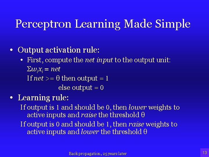
Perceptron Learning Made Simple • Output activation rule: • First, compute the net input to the output unit: Σwixi = net If net >= θ then output = 1 else output = 0 • Learning rule: If output is 1 and should be 0, then lower weights to active inputs and raise threshold θ If output is 0 and should be 1, then raise weights to active inputs and lower the threshold θ Back propagation, 25 years later 13

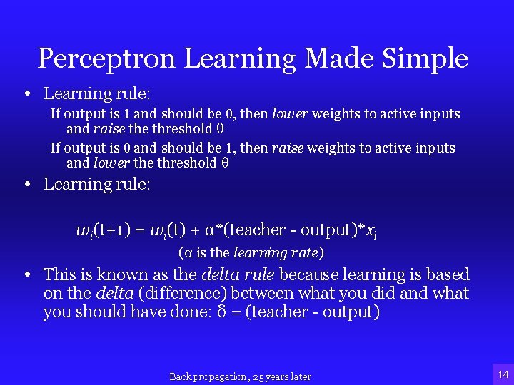
Perceptron Learning Made Simple • Learning rule: If output is 1 and should be 0, then lower weights to active inputs and raise threshold θ If output is 0 and should be 1, then raise weights to active inputs and lower the threshold θ • Learning rule: wi(t+1) = wi(t) + α*(teacher - output)*xi (α is the learning rate) • This is known as the delta rule because learning is based on the delta (difference) between what you did and what you should have done: δ = (teacher - output) Back propagation, 25 years later 14

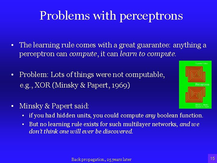
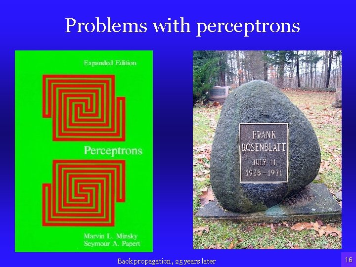
Problems with perceptrons • The learning rule comes with a great guarantee: anything a perceptron can compute, it can learn to compute. • Problem: Lots of things were not computable, e. g. , XOR (Minsky & Papert, 1969) • Minsky & Papert said: • if you had hidden units, you could compute any boolean function. • But no learning rule exists for such multilayer networks, and we don’t think one will ever be discovered. Back propagation, 25 years later 15

Problems with perceptrons Back propagation, 25 years later 16

Aside about perceptrons • They didn’t have hidden units - but Rosenblatt assumed nonlinear preprocessing! • Hidden units compute features of the input • The nonlinear preprocessing is a way to choose features by hand. • Support Vector Machines essentially do this in a principled way, followed by a (highly sophisticated) perceptron learning algorithm. Back propagation, 25 years later 17

Enter Rumelhart, Hinton, & Williams (1985) • Discovered a learning rule for networks with hidden units. • Works a lot like the perceptron algorithm: • • Randomly choose an input-output pattern present the input, let activation propagate through the network give the teaching signal propagate the error back through the network (hence the name back propagation) • change the connection strengths according to the error Back propagation, 25 years later 18

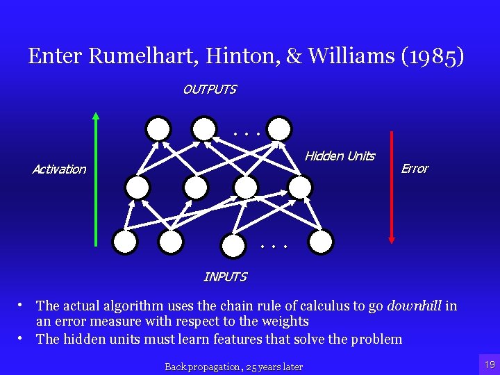
Enter Rumelhart, Hinton, & Williams (1985) OUTPUTS . . . Hidden Units Activation Error . . . INPUTS • The actual algorithm uses the chain rule of calculus to go downhill in an error measure with respect to the weights • The hidden units must learn features that solve the problem Back propagation, 25 years later 19

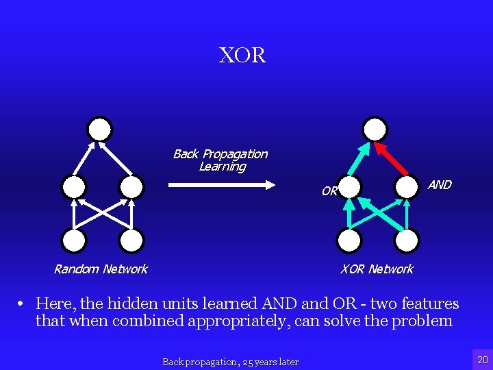
XOR Back Propagation Learning AND OR Random Network XOR Network • Here, the hidden units learned AND and OR - two features that when combined appropriately, can solve the problem Back propagation, 25 years later 20

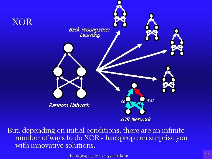
XOR Back Propagation Learning Random Network OR AND XOR Network But, depending on initial conditions, there an infinite number of ways to do XOR - backprop can surprise you with innovative solutions. Back propagation, 25 years later 21

Why is/was this wonderful? • • • Learns internal representations Efficient Generalizes to recurrent networks Back propagation, 25 years later 22

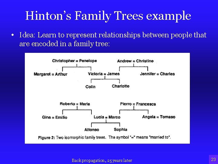
Hinton’s Family Trees example • Idea: Learn to represent relationships between people that are encoded in a family tree: Back propagation, 25 years later 23

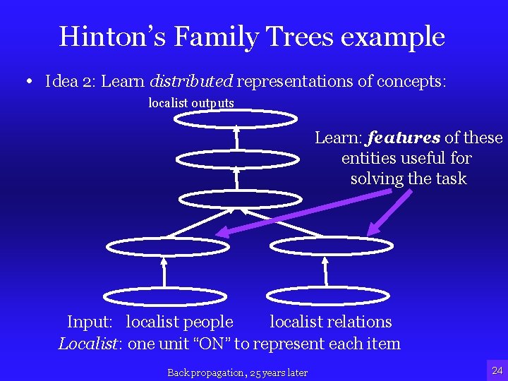
Hinton’s Family Trees example • Idea 2: Learn distributed representations of concepts: localist outputs Learn: features of these entities useful for solving the task Input: localist people localist relations Localist: one unit “ON” to represent each item Back propagation, 25 years later 24

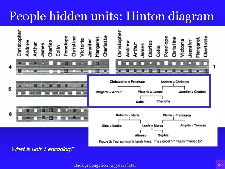
People hidden units: Hinton diagram • What does the unit 1 encode? What is unit 1 encoding? Back propagation, 25 years later 25

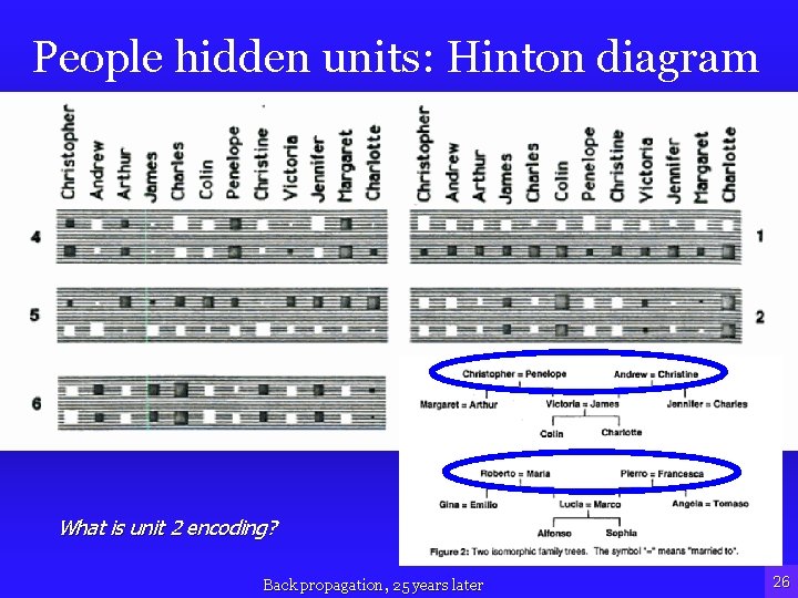
People hidden units: Hinton diagram • What does unit 2 encode? What is unit 2 encoding? Back propagation, 25 years later 26

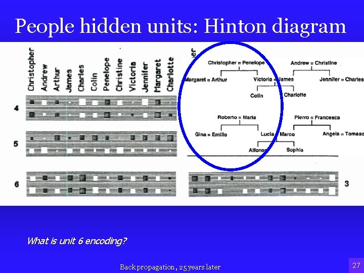
People hidden units: Hinton diagram • Unit 6? What is unit 6 encoding? Back propagation, 25 years later 27

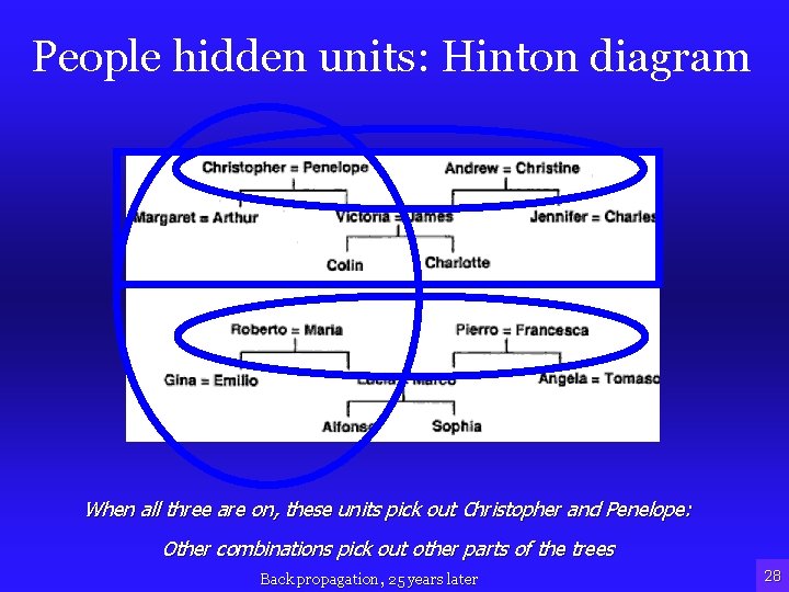
People hidden units: Hinton diagram When all three are on, these units pick out Christopher and Penelope: Other combinations pick out other parts of the trees Back propagation, 25 years later 28

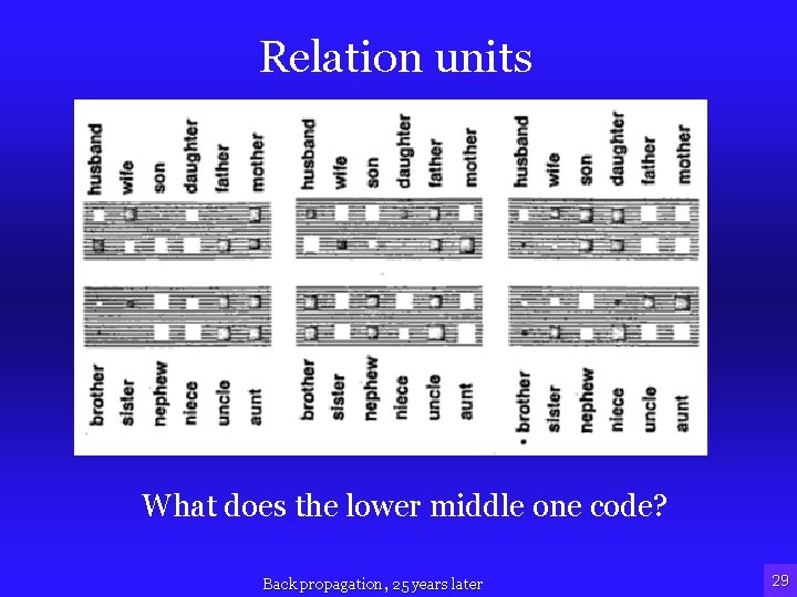
Relation units What does the lower middle one code? Back propagation, 25 years later 29

Lessons • The network learns features in the service of the task - i. e. , it learns features on its own. • This is useful if we don’t know what the features ought to be. • Can explain some human phenomena Back propagation, 25 years later 30

Another example • In the next example(s), I make two points: • The perceptron algorithm is still useful! • Representations learned in the service of the task can explain the “Visual Expertise Mystery” Back propagation, 25 years later 31

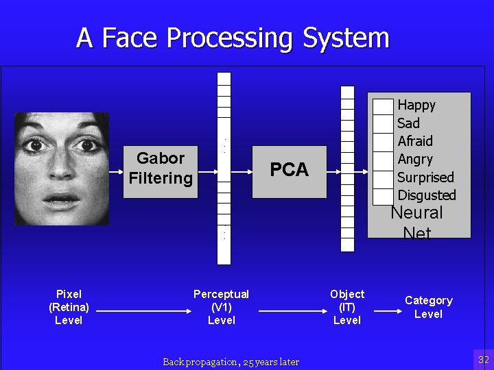
A Face Processing System Gabor Filtering Happy Sad Afraid Angry Surprised Disgusted . . . PCA Neural Net . . . Pixel (Retina) Level Perceptual (V 1) Level Back propagation, 25 years later Object (IT) Level Category Level 32

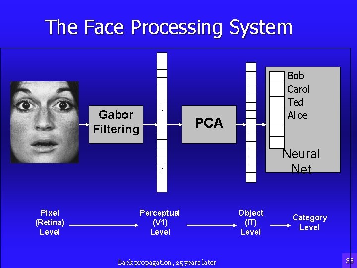
The Face Processing System Gabor Filtering Bob Carol Ted Alice . . . PCA Neural Net . . . Pixel (Retina) Level Perceptual (V 1) Level Back propagation, 25 years later Object (IT) Level Category Level 33

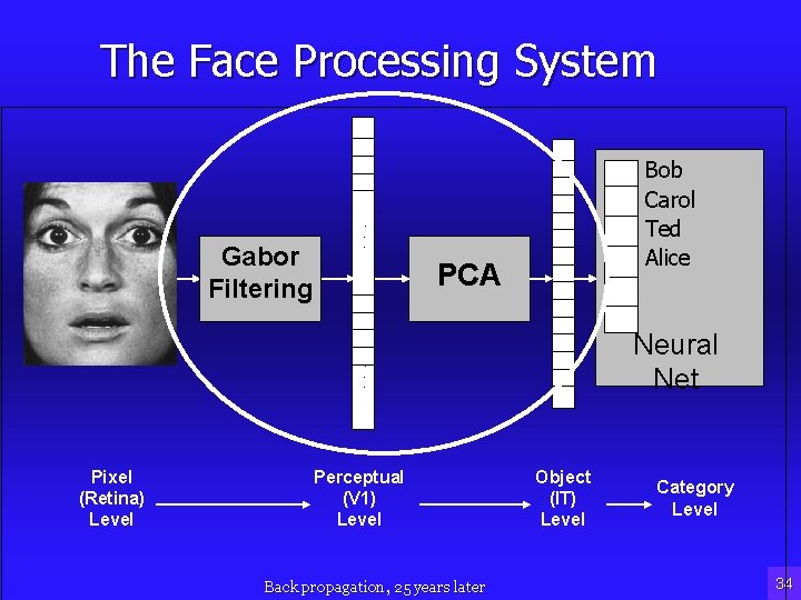
The Face Processing System Gabor Filtering Bob Carol Ted Alice . . . PCA Neural Net . . . Pixel (Retina) Level Perceptual (V 1) Level Back propagation, 25 years later Object (IT) Level Category Level 34

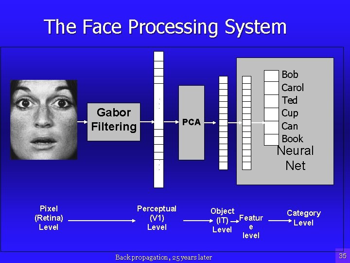
The Face Processing System Gabor Filtering Bob Carol Ted Cup Can Book . . . PCA Neural Net . . . Pixel (Retina) Level Perceptual (V 1) Level Object (IT) Featur e Level level Back propagation, 25 years later Category Level 35

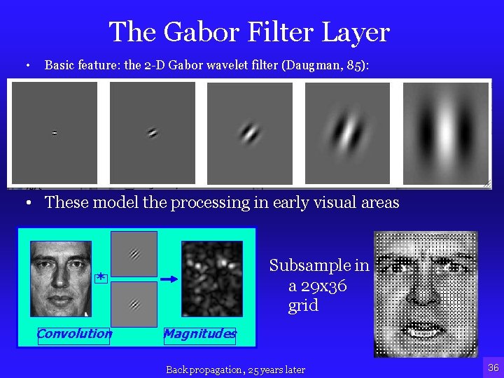
The Gabor Filter Layer • Basic feature: the 2 -D Gabor wavelet filter (Daugman, 85): • These model the processing in early visual areas Subsample in a 29 x 36 grid * Convolution Magnitudes Back propagation, 25 years later 36

Principal Components Analysis • The Gabor filters give us 40, 600 numbers • We use PCA to reduce this to 50 numbers • PCA is like Factor Analysis: It finds the underlying directions of Maximum Variance • PCA can be computed in a neural network through a competitive Hebbian learning mechanism • Hence this is also a biologically plausible processing step • We suggest this leads to representations similar to those in Inferior Temporal cortex Back propagation, 25 years later 37

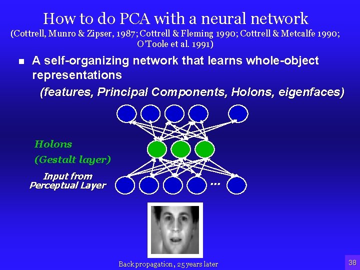
How to do PCA with a neural network (Cottrell, Munro & Zipser, 1987; Cottrell & Fleming 1990; Cottrell & Metcalfe 1990; O’Toole et al. 1991) n A self-organizing network that learns whole-object representations (features, Principal Components, Holons, eigenfaces) Holons (Gestalt layer) Input from Perceptual Layer . . . Back propagation, 25 years later 38

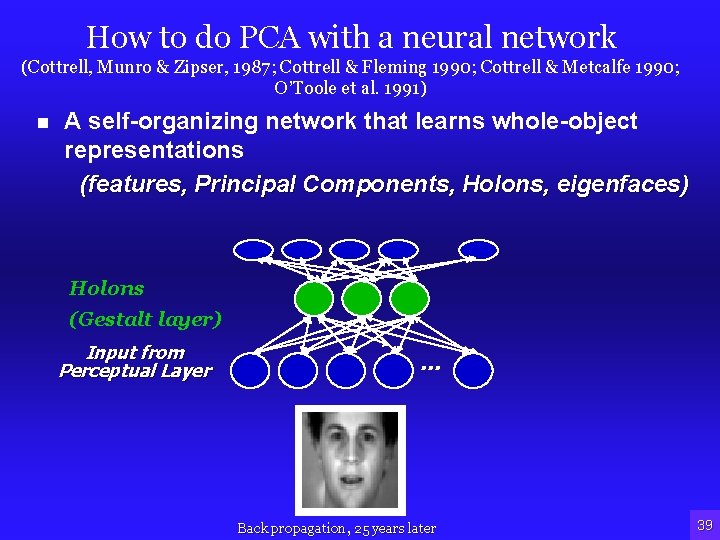
How to do PCA with a neural network (Cottrell, Munro & Zipser, 1987; Cottrell & Fleming 1990; Cottrell & Metcalfe 1990; O’Toole et al. 1991) n A self-organizing network that learns whole-object representations (features, Principal Components, Holons, eigenfaces) Holons (Gestalt layer) Input from Perceptual Layer . . . Back propagation, 25 years later 39

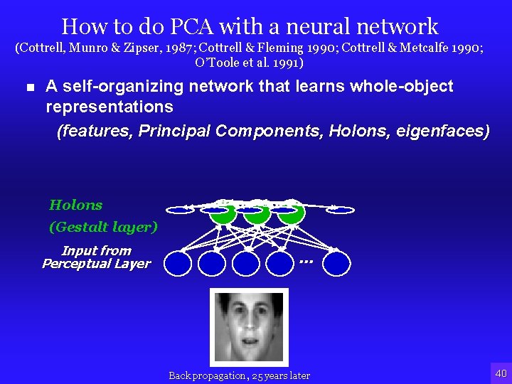
How to do PCA with a neural network (Cottrell, Munro & Zipser, 1987; Cottrell & Fleming 1990; Cottrell & Metcalfe 1990; O’Toole et al. 1991) n A self-organizing network that learns whole-object representations (features, Principal Components, Holons, eigenfaces) Holons (Gestalt layer) Input from Perceptual Layer . . . Back propagation, 25 years later 40

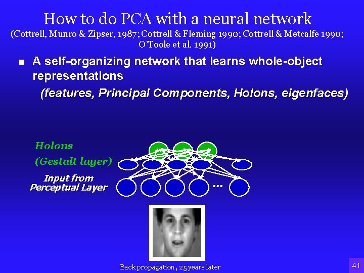
How to do PCA with a neural network (Cottrell, Munro & Zipser, 1987; Cottrell & Fleming 1990; Cottrell & Metcalfe 1990; O’Toole et al. 1991) n A self-organizing network that learns whole-object representations (features, Principal Components, Holons, eigenfaces) Holons (Gestalt layer) Input from Perceptual Layer . . . Back propagation, 25 years later 41

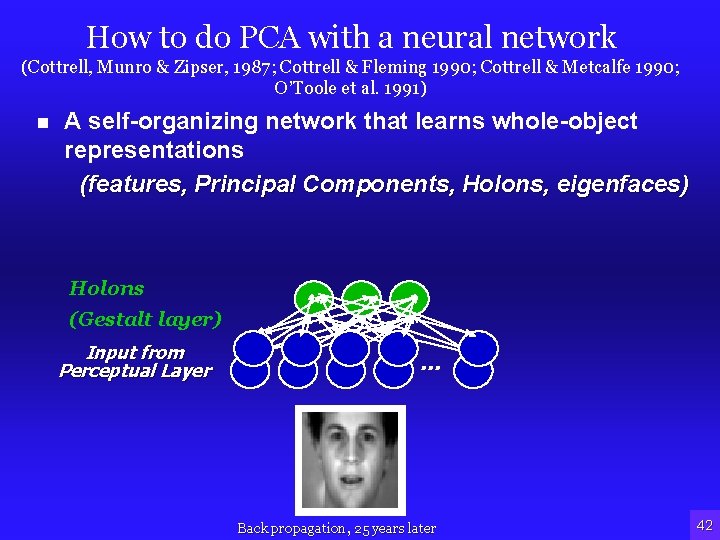
How to do PCA with a neural network (Cottrell, Munro & Zipser, 1987; Cottrell & Fleming 1990; Cottrell & Metcalfe 1990; O’Toole et al. 1991) n A self-organizing network that learns whole-object representations (features, Principal Components, Holons, eigenfaces) Holons (Gestalt layer) Input from Perceptual Layer . . . Back propagation, 25 years later 42

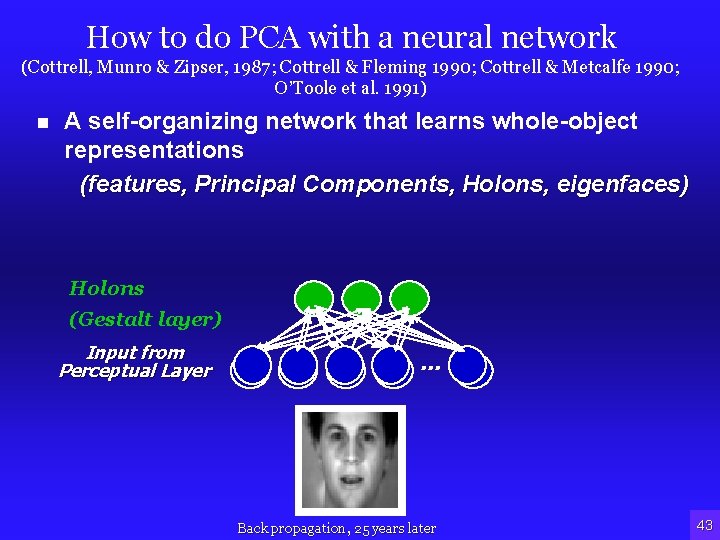
How to do PCA with a neural network (Cottrell, Munro & Zipser, 1987; Cottrell & Fleming 1990; Cottrell & Metcalfe 1990; O’Toole et al. 1991) n A self-organizing network that learns whole-object representations (features, Principal Components, Holons, eigenfaces) Holons (Gestalt layer) Input from Perceptual Layer . . . Back propagation, 25 years later 43

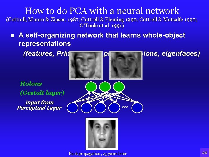
How to do PCA with a neural network (Cottrell, Munro & Zipser, 1987; Cottrell & Fleming 1990; Cottrell & Metcalfe 1990; O’Toole et al. 1991) n A self-organizing network that learns whole-object representations (features, Principal Components, Holons, eigenfaces) Holons (Gestalt layer) Input from Perceptual Layer . . . Back propagation, 25 years later 44

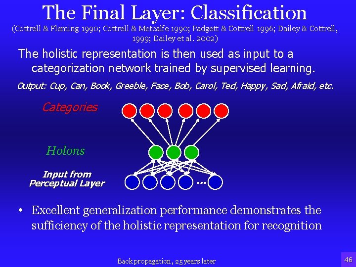
The Final Layer: Classification (Cottrell & Fleming 1990; Cottrell & Metcalfe 1990; Padgett & Cottrell 1996; Dailey & Cottrell, 1999; Dailey et al. 2002) The holistic representation is then used as input to a categorization network trained by supervised learning. Output: Cup, Can, Book, Greeble, Face, Bob, Carol, Ted, Happy, Sad, Afraid, etc. Categories Holons Input from Perceptual Layer . . . • Excellent generalization performance demonstrates the sufficiency of the holistic representation for recognition Back propagation, 25 years later 46

The Final Layer: Classification • Categories can be at different levels: basic, subordinate. • Simple learning rule (~delta rule). It says (mild lie here): • add inputs to your weights (synaptic strengths) when you are supposed to be on, • subtract them when you are supposed to be off. • This makes your weights “look like” your favorite patterns – the ones that turn you on. • When no hidden units => No back propagation of error. • When hidden units: we get task-specific features (most interesting when we use the basic/subordinate distinction) Back propagation, 25 years later 47

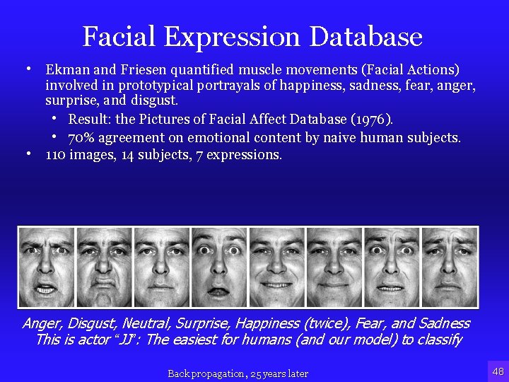
Facial Expression Database • Ekman and Friesen quantified muscle movements (Facial Actions) involved in prototypical portrayals of happiness, sadness, fear, anger, surprise, and disgust. • Result: the Pictures of Facial Affect Database (1976). • 70% agreement on emotional content by naive human subjects. • 110 images, 14 subjects, 7 expressions. Anger, Disgust, Neutral, Surprise, Happiness (twice), Fear, and Sadness This is actor “JJ”: The easiest for humans (and our model) to classify Back propagation, 25 years later 48

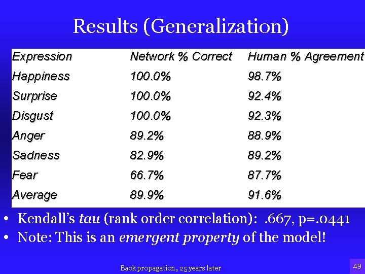
Results (Generalization) Expression Network % Correct Human % Agreement Happiness 100. 0% 98. 7% Surprise 100. 0% 92. 4% Disgust 100. 0% 92. 3% Anger 89. 2% 88. 9% Sadness 82. 9% 89. 2% Fear 66. 7% 87. 7% Average 89. 9% 91. 6% • Kendall’s tau (rank order correlation): . 667, p=. 0441 • Note: This is an emergent property of the model! Back propagation, 25 years later 49

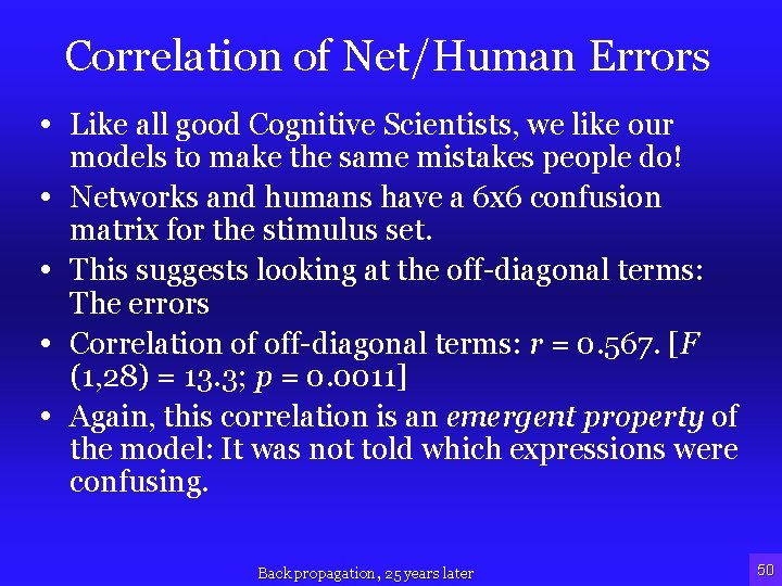
Correlation of Net/Human Errors • Like all good Cognitive Scientists, we like our • • models to make the same mistakes people do! Networks and humans have a 6 x 6 confusion matrix for the stimulus set. This suggests looking at the off-diagonal terms: The errors Correlation of off-diagonal terms: r = 0. 567. [F (1, 28) = 13. 3; p = 0. 0011] Again, this correlation is an emergent property of the model: It was not told which expressions were confusing. Back propagation, 25 years later 50

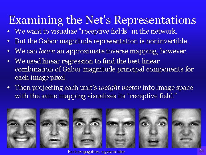
Examining the Net’s Representations • • We want to visualize “receptive fields” in the network. But the Gabor magnitude representation is noninvertible. We can learn an approximate inverse mapping, however. We used linear regression to find the best linear combination of Gabor magnitude principal components for each image pixel. • Then projecting each unit’s weight vector into image space with the same mapping visualizes its “receptive field. ” Back propagation, 25 years later 51

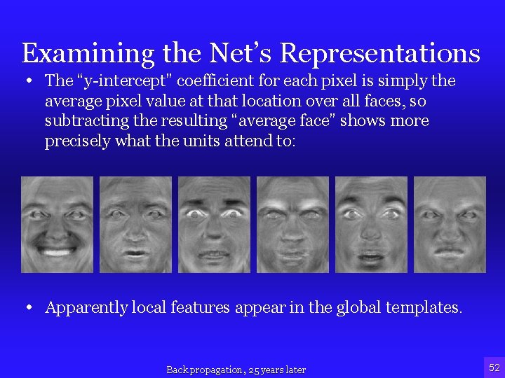
Examining the Net’s Representations • The “y-intercept” coefficient for each pixel is simply the average pixel value at that location over all faces, so subtracting the resulting “average face” shows more precisely what the units attend to: • Apparently local features appear in the global templates. Back propagation, 25 years later 52

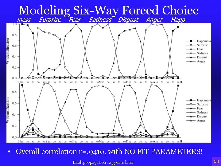
Modeling Six-Way Forced Choice iness Surprise Fear Sadness Disgust Anger Happ- • Overall correlation r=. 9416, with NO FIT PARAMETERS! Back propagation, 25 years later 58

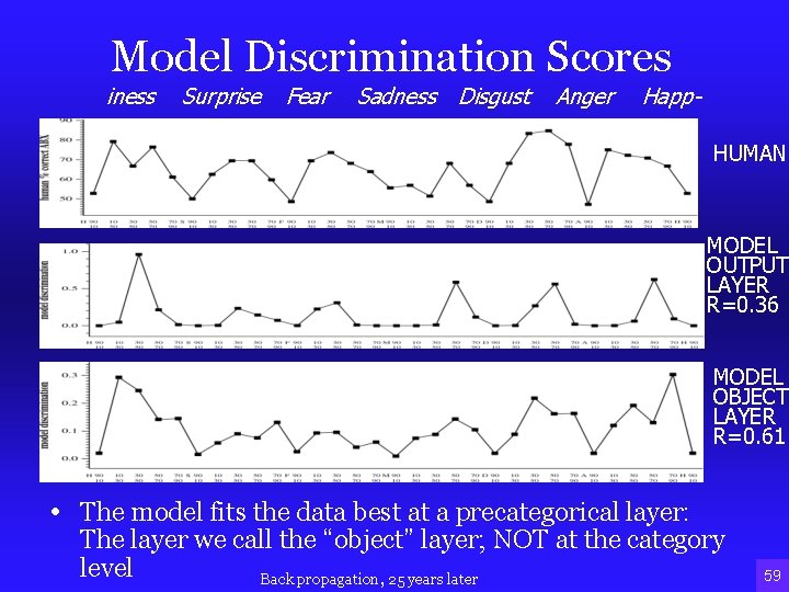
Model Discrimination Scores iness Surprise Fear Sadness Disgust Anger Happ. HUMAN MODEL OUTPUT LAYER R=0. 36 PERCENT CORRECT DISCRIMINATION MODEL OBJECT LAYER R=0. 61 • The model fits the data best at a precategorical layer: The layer we call the “object” layer; NOT at the category level Back propagation, 25 years later 59

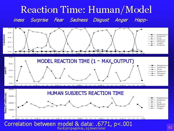
Reaction Time: Human/Model iness Surprise Fear Sadness Disgust Anger Happ- MODEL REACTION TIME (1 - MAX_OUTPUT) HUMAN SUBJECTS REACTION TIME Correlation between model & data: . 6771, p<. 001 Back propagation, 25 years later 62

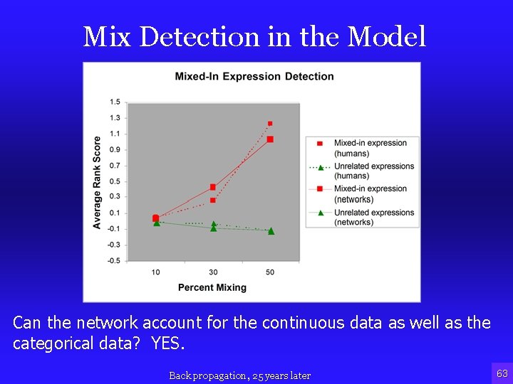
Mix Detection in the Model Can the network account for the continuous data as well as the categorical data? YES. Back propagation, 25 years later 63

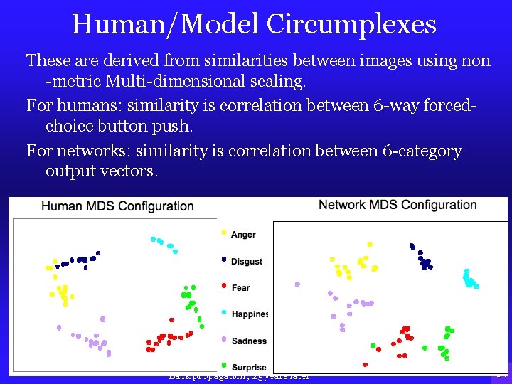
Human/Model Circumplexes These are derived from similarities between images using non -metric Multi-dimensional scaling. For humans: similarity is correlation between 6 -way forcedchoice button push. For networks: similarity is correlation between 6 -category output vectors. Back propagation, 25 years later 64

Discussion • Our model of facial expression recognition: • Performs the same task people do • On the same stimuli • At about the same accuracy • Without actually “feeling” anything, without any access to the surrounding culture, it nevertheless: • Organizes the faces in the same order around the circumplex • Correlates very highly with human responses. • Has about the same rank order difficulty in classifying the emotions Back propagation, 25 years later 66

Backprop, 25 years later • Backprop is important because it was the first relatively efficient method for learning internal representations • Recent advances have made deeper networks possible • This is important because we don’t know how the brain uses transformations to recognize objects across a wide array of variations (e. g. , the Halle Berry neuron) Back propagation, 25 years later 69

END 70

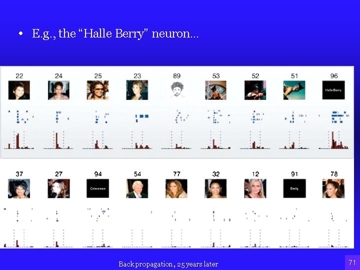
• E. g. , the “Halle Berry” neuron… Back propagation, 25 years later 71