Back to George One More Time Before they

Back to George One More Time • Before they invented drawing boards, what did they go back to? • If all the world is a stage, where is the audience sitting? • If the #2 pencil is the most popular, why is it still #2? • If work is so terrific, how come they have to pay you to do it? • If you ate pasta and antipasto, would you still be hungry? • If you try to fail, and succeed, which have you done? • "People who think they know everything are a great annoyance to those of us who do. ” - Anon
O() Analysis Reasonable vs. Unreasonable Algorithms Using O() Analysis in Design Concurrent Systems Parallelism
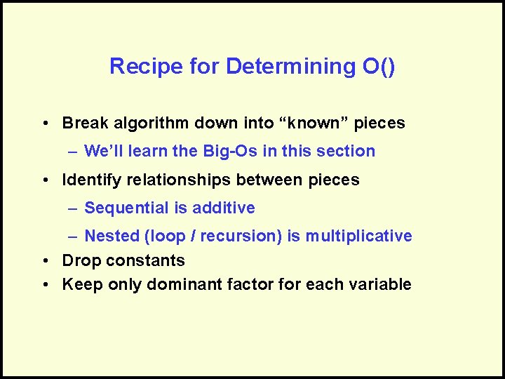
Recipe for Determining O() • Break algorithm down into “known” pieces – We’ll learn the Big-Os in this section • Identify relationships between pieces – Sequential is additive – Nested (loop / recursion) is multiplicative • Drop constants • Keep only dominant factor for each variable
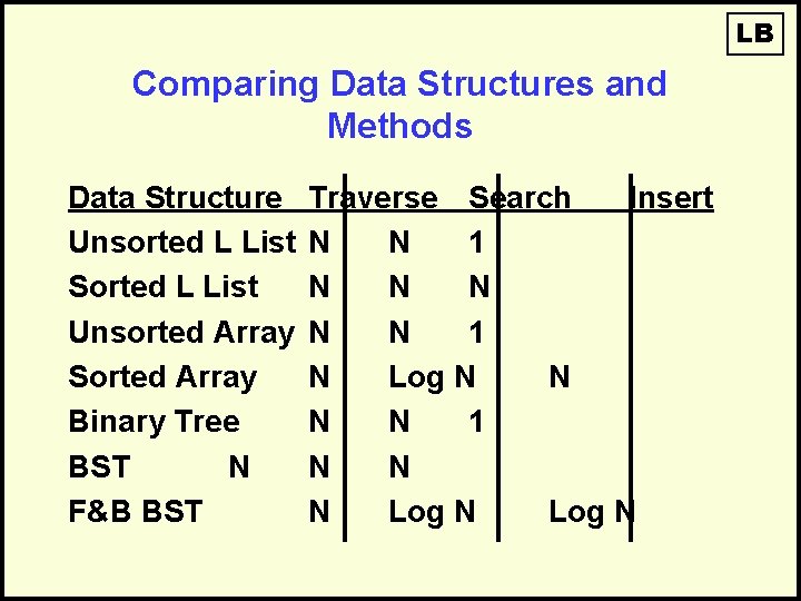
LB Comparing Data Structures and Methods Data Structure Unsorted L List Sorted L List Unsorted Array Sorted Array Binary Tree BST N F&B BST Traverse Search Insert N N 1 N Log N N 1 N N N Log N
Reasonable vs. Unreasonable Algorithms
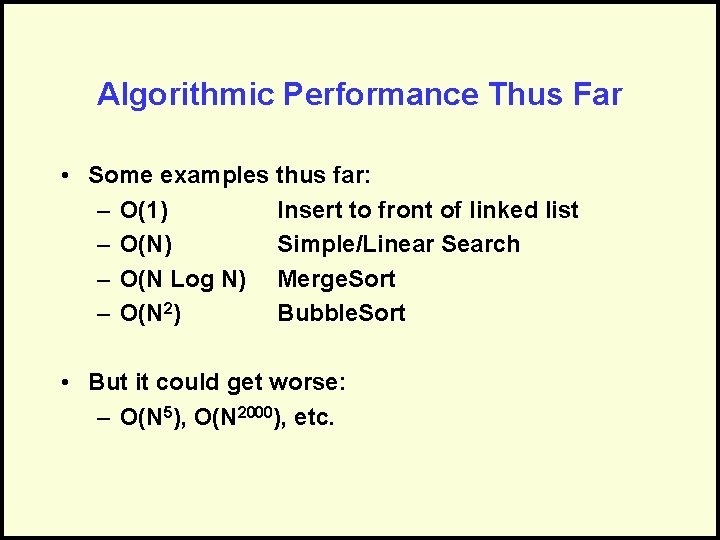
Algorithmic Performance Thus Far • Some examples thus far: – O(1) Insert to front of linked list – O(N) Simple/Linear Search – O(N Log N) Merge. Sort – O(N 2) Bubble. Sort • But it could get worse: – O(N 5), O(N 2000), etc.
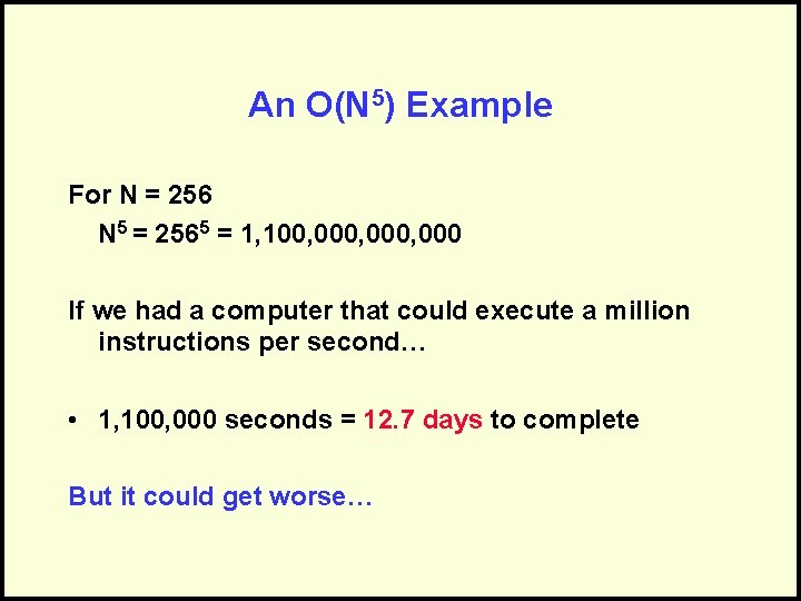
An O(N 5) Example For N = 256 N 5 = 2565 = 1, 100, 000, 000 If we had a computer that could execute a million instructions per second… • 1, 100, 000 seconds = 12. 7 days to complete But it could get worse…
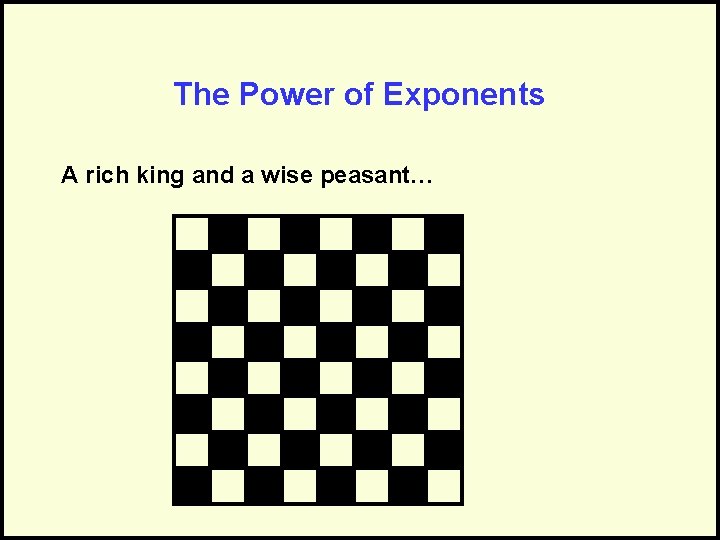
The Power of Exponents A rich king and a wise peasant…
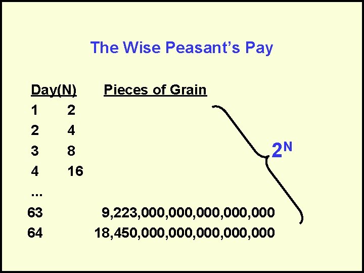
The Wise Peasant’s Pay Day(N) Pieces of Grain 1 2 2 4 3 8 2 N 4 16. . . 63 9, 223, 000, 000 64 18, 450, 000, 000
How Bad is 2 N? • Imagine being able to grow a billion (1, 000, 000) pieces of grain a second… • It would take – 585 years to grow enough grain just for the 64 th day – Over a thousand years to fulfill the peasant’s request!

LB So the King cut off the peasant’s head.
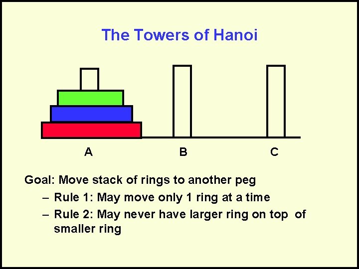
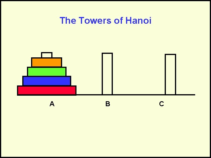
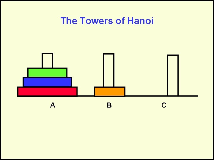
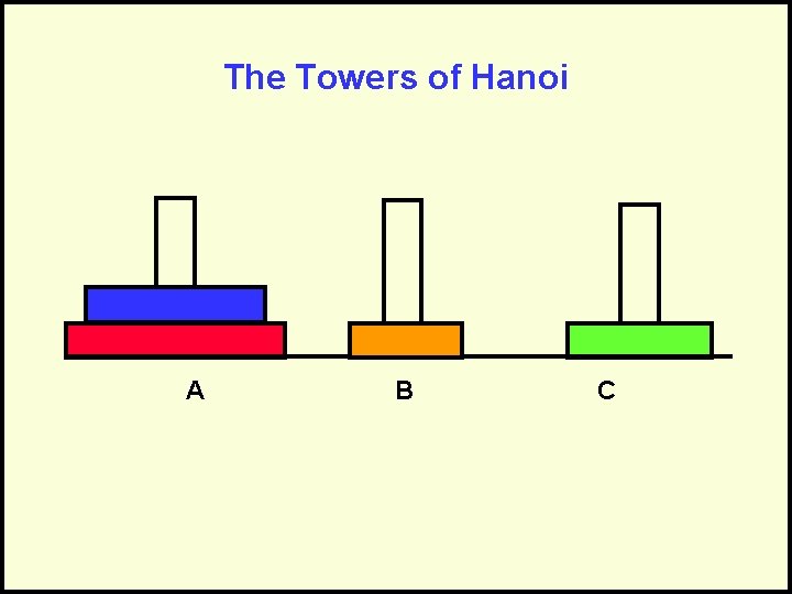
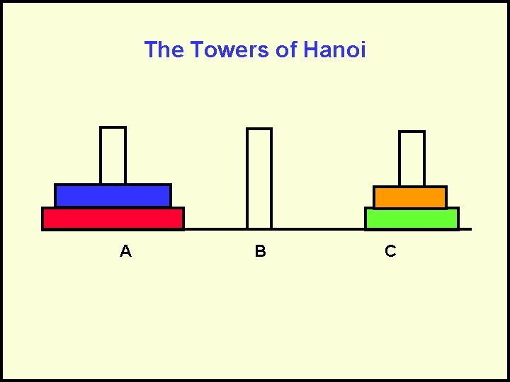
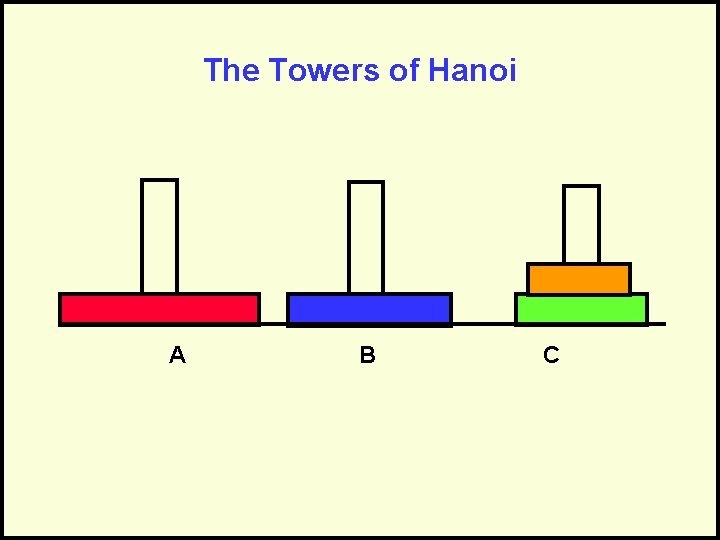
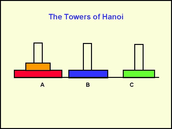
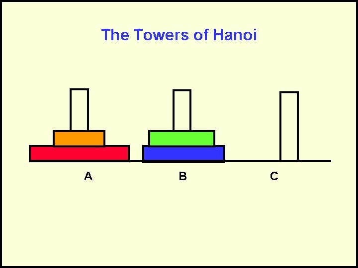
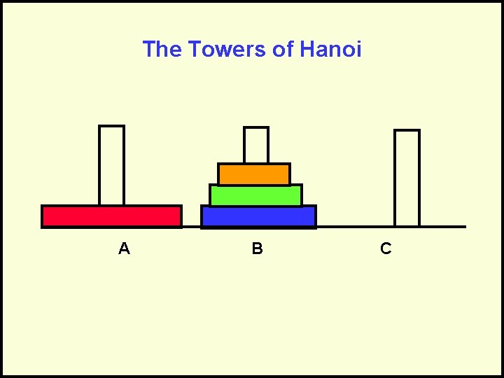
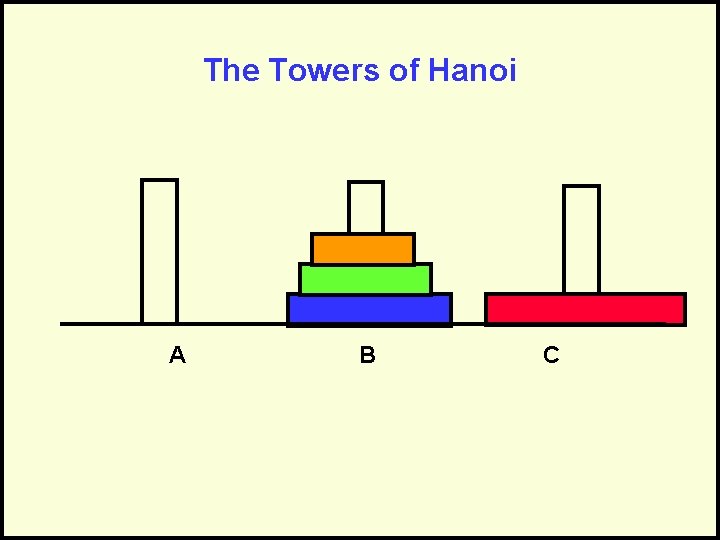
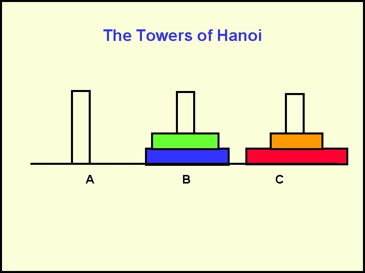
The Towers of Hanoi A B C Goal: Move stack of rings to another peg – Rule 1: May move only 1 ring at a time – Rule 2: May never have larger ring on top of smaller ring
The Towers of Hanoi A B C
The Towers of Hanoi A B C
The Towers of Hanoi A B C
The Towers of Hanoi A B C
The Towers of Hanoi A B C
The Towers of Hanoi A B C
The Towers of Hanoi A B C
The Towers of Hanoi A B C
The Towers of Hanoi A B C
The Towers of Hanoi A B C
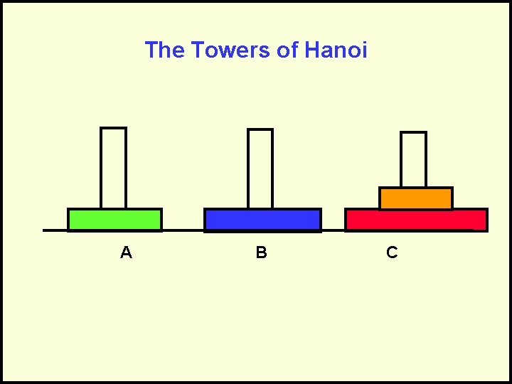
The Towers of Hanoi A B C
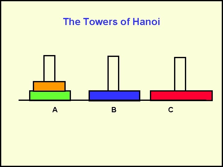
The Towers of Hanoi A B C
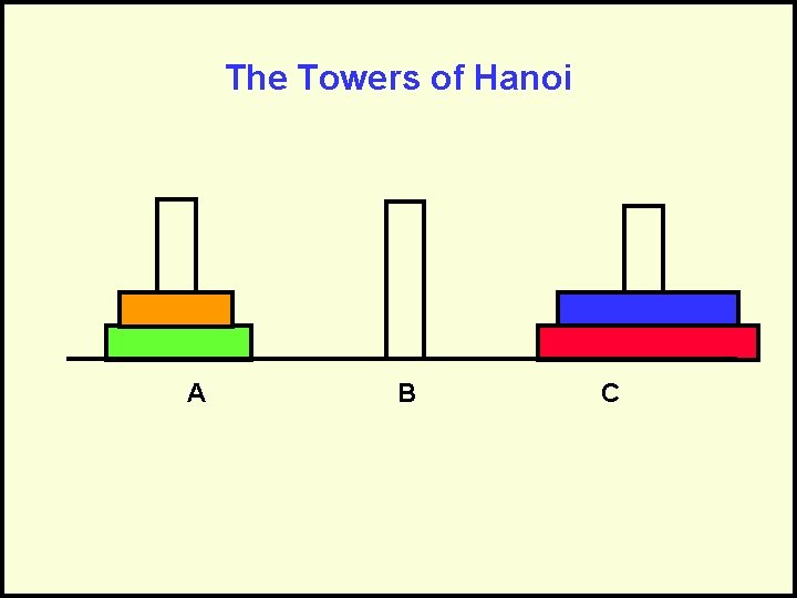
The Towers of Hanoi A B C
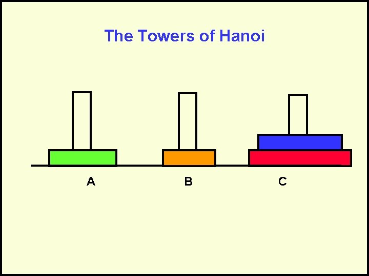
The Towers of Hanoi A B C
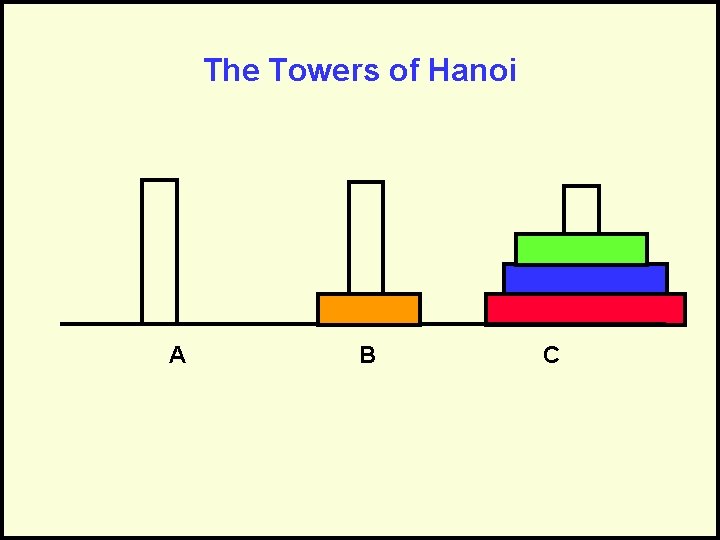
The Towers of Hanoi A B C
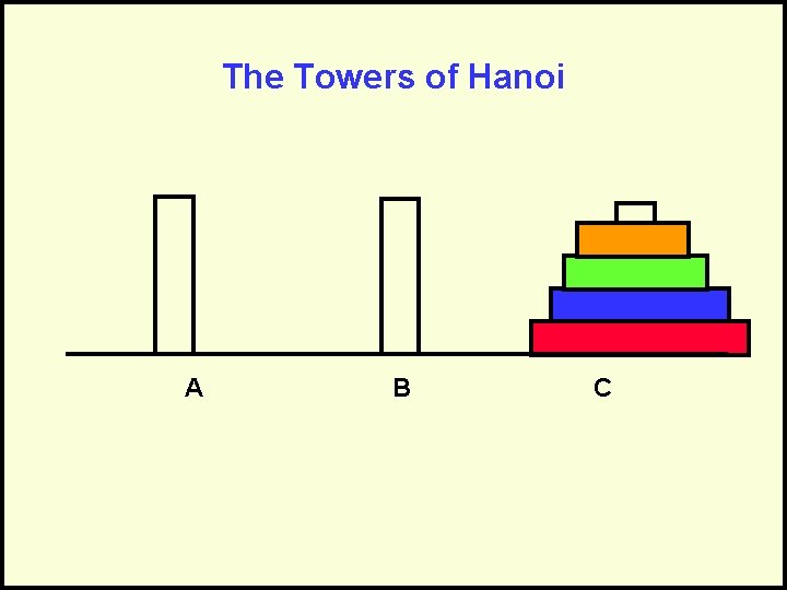
The Towers of Hanoi A B C
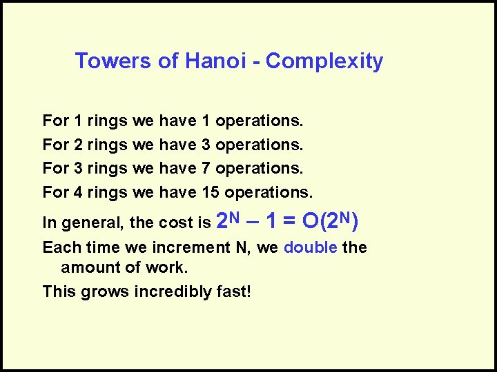
Towers of Hanoi - Complexity For 1 rings we have 1 operations. For 2 rings we have 3 operations. For 3 rings we have 7 operations. For 4 rings we have 15 operations. In general, the cost is 2 N – 1 = O(2 N) Each time we increment N, we double the amount of work. This grows incredibly fast!
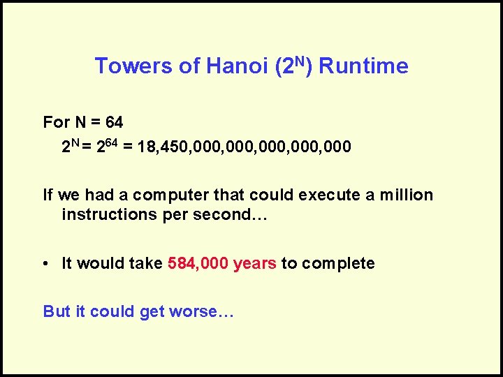
Towers of Hanoi (2 N) Runtime For N = 64 2 N = 264 = 18, 450, 000, 000 If we had a computer that could execute a million instructions per second… • It would take 584, 000 years to complete But it could get worse…
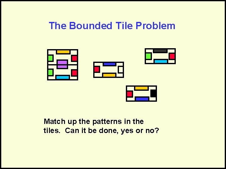
The Bounded Tile Problem Match up the patterns in the tiles. Can it be done, yes or no?
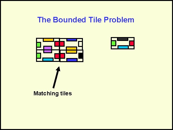
The Bounded Tile Problem Matching tiles
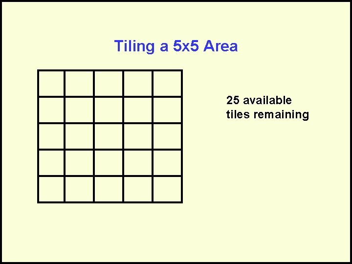
Tiling a 5 x 5 Area 25 available tiles remaining
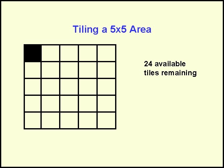
Tiling a 5 x 5 Area 24 available tiles remaining
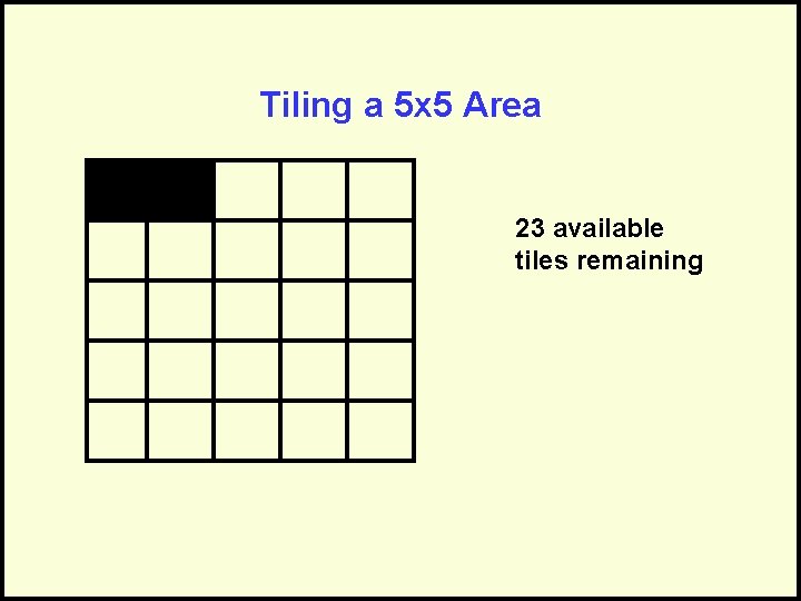
Tiling a 5 x 5 Area 23 available tiles remaining
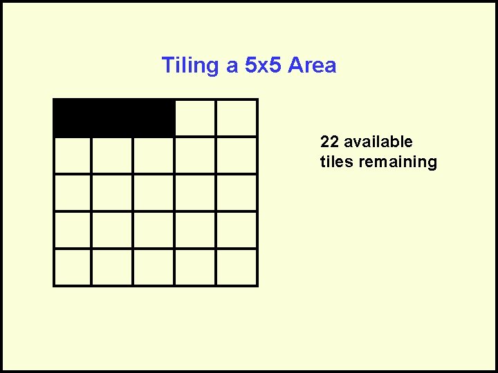
Tiling a 5 x 5 Area 22 available tiles remaining
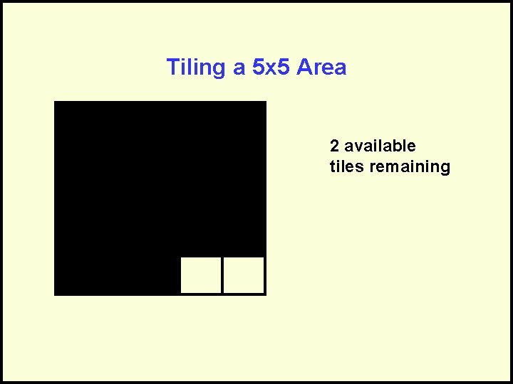
Tiling a 5 x 5 Area 2 available tiles remaining
Analysis of the Bounded Tiling Problem Tile a 5 by 5 area (N = 25 tiles) 1 st location: 25 choices 2 nd location: 24 choices And so on… Total number of arrangements: – 25 * 24 * 23 * 22 * 21 *. . * 3 * 2 * 1 – 25! (Factorial) = 15, 500, 000, 000, 000 Bounded Tiling Problem is O(N!)
Tiling (N!) Runtime For N = 25 25! = 15, 500, 000, 000, 000 If we could “place” a million tiles per second… • It would take 470 billion years to complete Why not a faster computer?
A Faster Computer • If we had a computer that could execute a trillion instructions per second (a million times faster than our MIPS computer)… • 5 x 5 tiling problem would take 470, 000 years • 64 -ring Tower of Hanoi problem would take 213 days Why not an even faster computer!
The Fastest Computer Possible? • What if: – Instructions took ZERO time to execute – CPU registers could be loaded at the speed of light • These algorithms are still unreasonable! • The speed of light is only so fast!
Where Does this Leave Us? • Clearly algorithms have varying runtimes. • We’d like a way to categorize them: – Reasonable, so it may be useful – Unreasonable, so why bother running
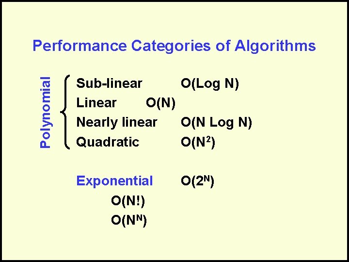
Polynomial Performance Categories of Algorithms Sub-linear O(Log N) Linear O(N) Nearly linear O(N Log N) Quadratic O(N 2) Exponential O(N!) O(NN) O(2 N)
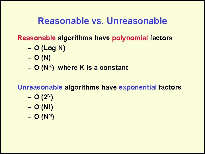
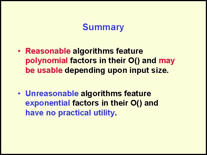
Reasonable vs. Unreasonable Reasonable algorithms have polynomial factors – O (Log N) – O (NK) where K is a constant Unreasonable algorithms have exponential factors – O (2 N) – O (N!) – O (NN)
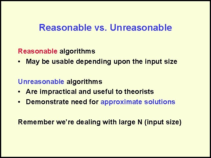
Reasonable vs. Unreasonable Reasonable algorithms • May be usable depending upon the input size Unreasonable algorithms • Are impractical and useful to theorists • Demonstrate need for approximate solutions Remember we’re dealing with large N (input size)
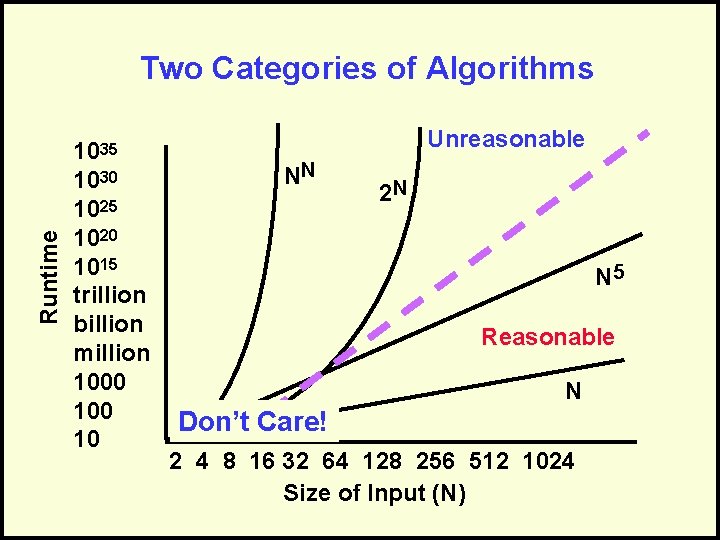
Runtime Two Categories of Algorithms 1035 1030 1025 1020 1015 trillion billion million 1000 10 Unreasonable NN 2 N N 5 Reasonable N Don’t Care! 2 4 8 16 32 64 128 256 512 1024 Size of Input (N)
Summary • Reasonable algorithms feature polynomial factors in their O() and may be usable depending upon input size. • Unreasonable algorithms feature exponential factors in their O() and have no practical utility.

Questions?

Using O() Analysis in Design
Air Traffic Control Conflict Alert Coast, add, delete
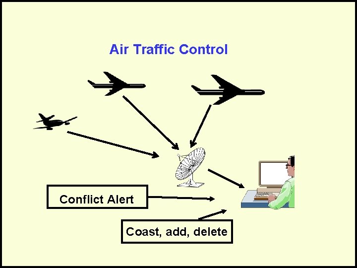
Problem Statement • What data structure should be used to store the aircraft records for this system? • Normal operations conducted are: – Data Entry: adding new aircraft entering the area – Radar Update: input from the antenna – Coast: global traversal to verify that all aircraft have been updated [coast for 5 cycles, then drop] – Query: controller requesting data about a specific aircraft by location – Conflict Analysis: make sure no two aircraft are too close together
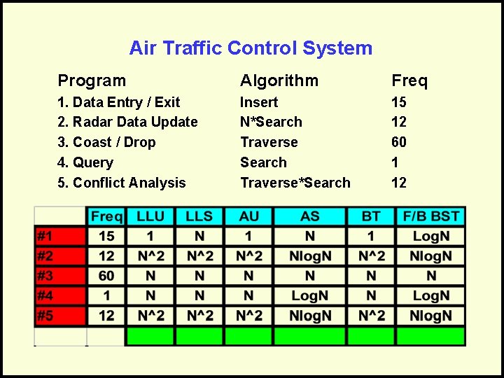
Air Traffic Control System Program Algorithm Freq 1. Data Entry / Exit 2. Radar Data Update 3. Coast / Drop 4. Query 5. Conflict Analysis Insert N*Search Traverse*Search 15 12 60 1 12

Questions?
Concurrent Systems
Sequential Processing • All of the algorithms we’ve seen so far are sequential: – They have one “thread” of execution – One step follows another in sequence – One processor is all that is needed to run the algorithm
A Non-sequential Example • Consider a house with a burglar alarm system. • The system continually monitors: – The front door – The back door – The sliding glass door – The door to the deck – The kitchen windows – The living room windows – The bedroom windows • The burglar alarm is watching all of these “at once” (at the same time).
Another Non-sequential Example • Your car has an onboard digital dashboard that simultaneously: – Calculates how fast you’re going and displays it on the speedometer – Checks your oil level – Checks your fuel level and calculates consumption – Monitors the heat of the engine and turns on a light if it is too hot – Monitors your alternator to make sure it is charging your battery
Concurrent Systems • A system in which: – Multiple tasks can be executed at the same time – The tasks may be duplicates of each other, or distinct tasks – The overall time to perform the series of tasks is reduced
Advantages of Concurrency • Concurrent processes can reduce duplication in code. • The overall runtime of the algorithm can be significantly reduced. • More real-world problems can be solved than with sequential algorithms alone. • Redundancy can make systems more reliable.
Disadvantages of Concurrency • Runtime is not always reduced, so careful planning is required • Concurrent algorithms can be more complex than sequential algorithms • Shared data can be corrupted • Communications between tasks is needed
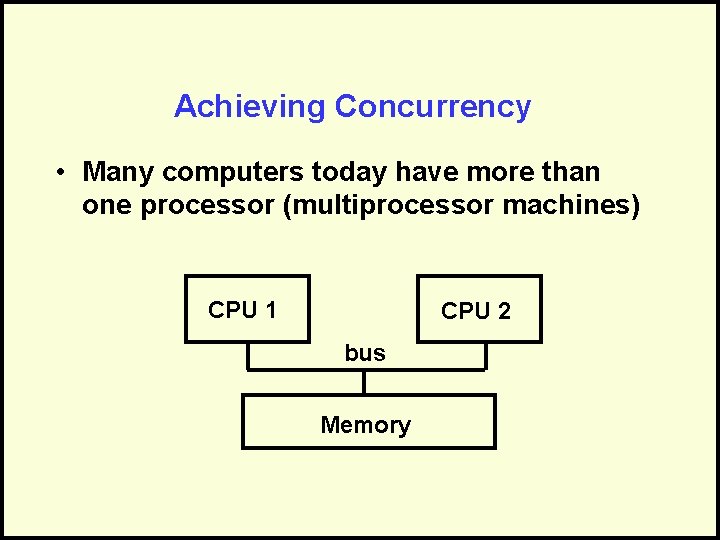
Achieving Concurrency • Many computers today have more than one processor (multiprocessor machines) CPU 1 CPU 2 bus Memory
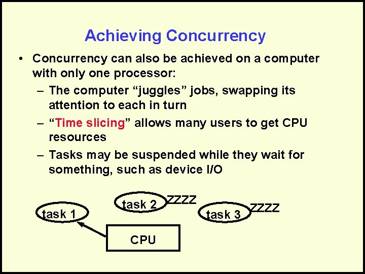
Achieving Concurrency • Concurrency can also be achieved on a computer with only one processor: – The computer “juggles” jobs, swapping its attention to each in turn – “Time slicing” allows many users to get CPU resources – Tasks may be suspended while they wait for something, such as device I/O task 1 task 2 ZZZZ CPU task 3 ZZZZ
Concurrency vs. Parallelism • Concurrency is the execution of multiple tasks at the same time, regardless of the number of processors. • Parallelism is the execution of multiple processors on the same task.
Types of Concurrent Systems • • Multiprogramming Multiprocessing Multitasking Distributed Systems
Multiprogramming • Share a single CPU among many users or tasks. • May have a time-shared algorithm or a priority algorithm for determining which task to run next • Give the illusion of simultaneous processing through rapid swapping of tasks (interleaving).
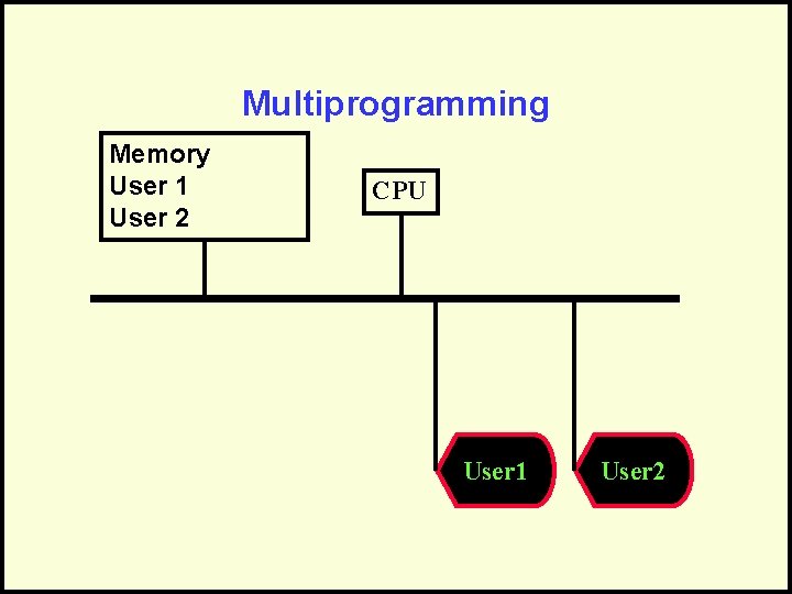
Multiprogramming Memory User 1 User 2 CPU User 1 User 2
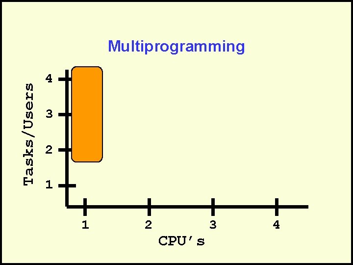
Tasks/Users Multiprogramming 4 3 2 1 1 2 CPU’s 3 4
Multiprocessing • Executes multiple tasks at the same time • Uses multiple processors to accomplish the tasks • Each processor may also timeshare among several tasks • Has a shared memory that is used by all the tasks
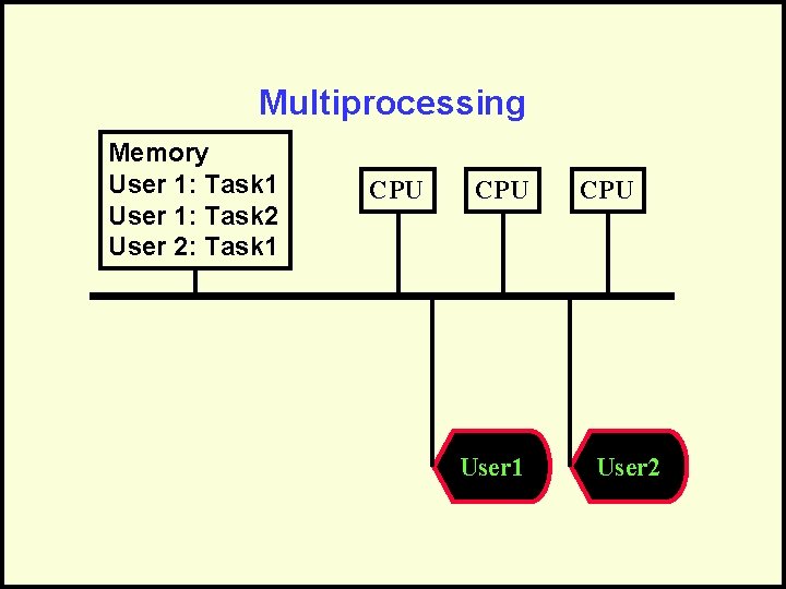
Multiprocessing Memory User 1: Task 1 User 1: Task 2 User 2: Task 1 CPU User 2
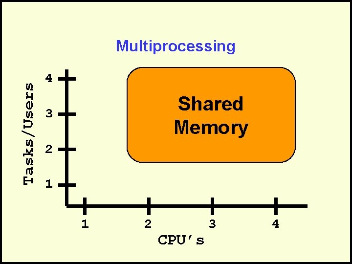
Tasks/Users Multiprocessing 4 Shared Memory 3 2 1 1 2 CPU’s 3 4
Multitasking • A single user can have multiple tasks running at the same time. • Can be done with one or more processors. • Used to be rare and for only expensive multiprocessing systems, but now most modern operating systems can do it.
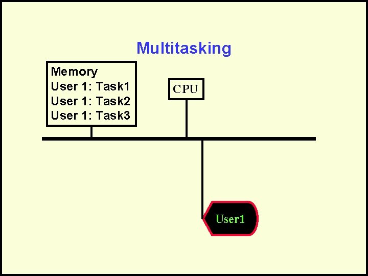
Multitasking Memory User 1: Task 1 User 1: Task 2 User 1: Task 3 CPU User 1
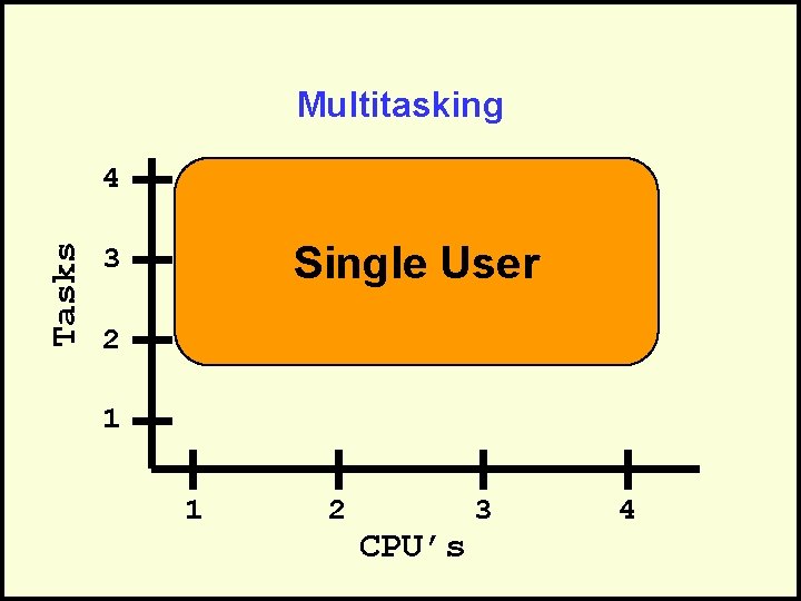
Multitasking Tasks 4 Single User 3 2 1 1 2 CPU’s 3 4
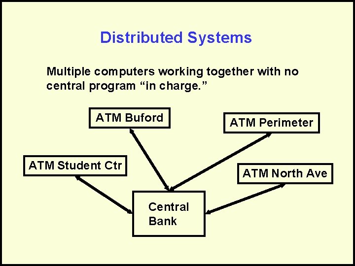
Distributed Systems Multiple computers working together with no central program “in charge. ” ATM Buford ATM Student Ctr ATM Perimeter ATM North Ave Central Bank
Distributed Systems • Advantages: – No bottlenecks from sharing processors – No central point of failure – Processing can be localized for efficiency • Disadvantages: – Complexity – Communication overhead – Distributed control

Questions?
Parallelism
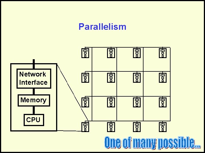
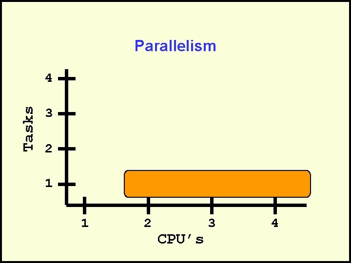
Parallelism • Using multiple processors to solve a single task. • Involves: – Breaking the task into meaningful pieces – Doing the work on many processors – Coordinating and putting the pieces back together.
Parallelism Network Interface Memory CPU
Parallelism Tasks 4 3 2 1 1 2 CPU’s 3 4
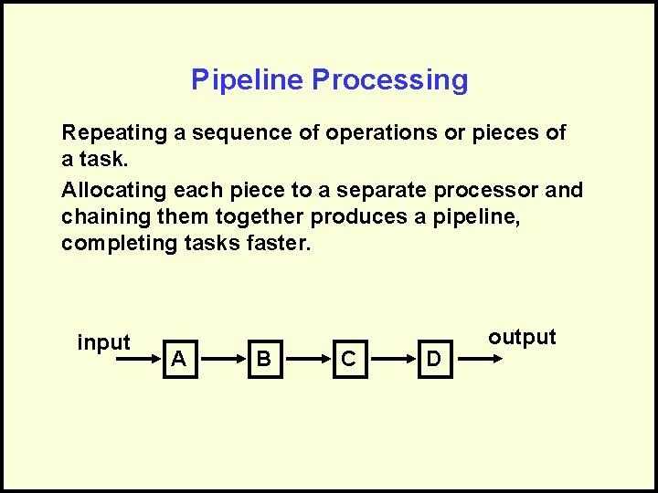
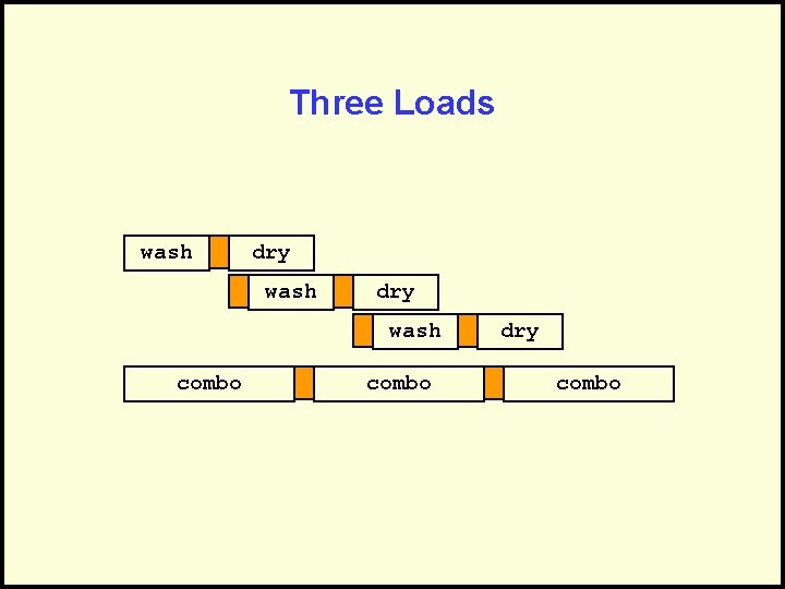
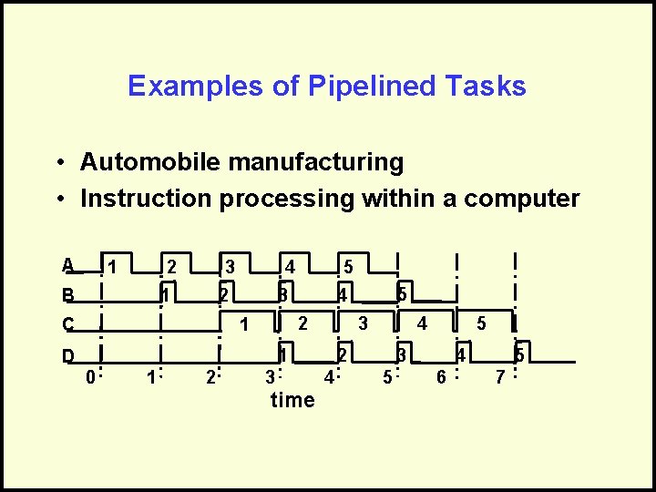
Pipeline Processing Repeating a sequence of operations or pieces of a task. Allocating each piece to a separate processor and chaining them together produces a pipeline, completing tasks faster. input A B C D output
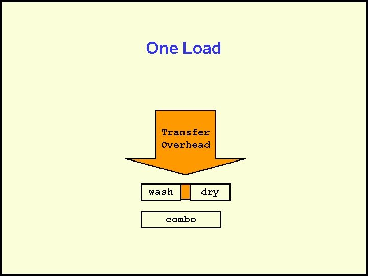
Example • Suppose you have a choice between a washer and a dryer each having a 30 minutes cycle or • A washer/dryer with a one hour cycle • The correct answer depends on how much work you have to do.
One Load Transfer Overhead wash combo dry
Three Loads wash dry wash combo dry combo
Examples of Pipelined Tasks • Automobile manufacturing • Instruction processing within a computer A 2 1 B 3 4 2 1 C 5 3 2 1 0 1 2 3 2 time 4 5 4 3 1 D 5 4 5 5 4 3 6 7
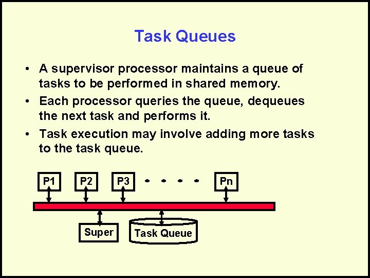
Task Queues • A supervisor processor maintains a queue of tasks to be performed in shared memory. • Each processor queries the queue, dequeues the next task and performs it. • Task execution may involve adding more tasks to the task queue. P 1 P 2 Super P 3 Pn Task Queue
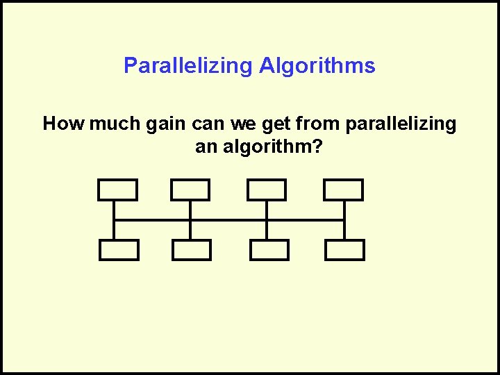
Parallelizing Algorithms How much gain can we get from parallelizing an algorithm?
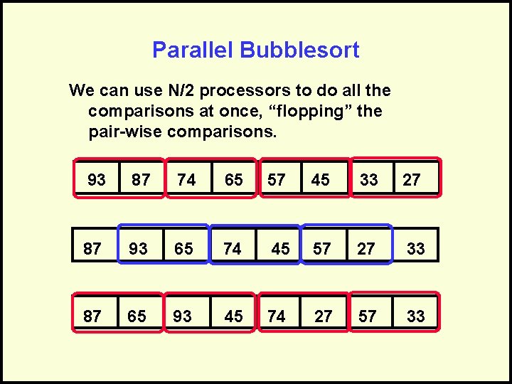
Parallel Bubblesort We can use N/2 processors to do all the comparisons at once, “flopping” the pair-wise comparisons. 93 87 74 65 57 45 33 27 87 93 65 74 45 57 27 33 87 65 93 45 74 27 57 33
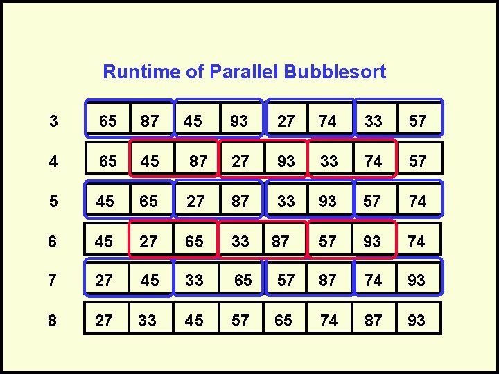
Runtime of Parallel Bubblesort 3 65 87 4 65 45 6 45 93 27 74 33 57 87 27 93 33 74 57 65 27 87 33 93 57 74 45 27 65 33 57 93 74 7 27 45 33 65 57 87 74 93 8 27 33 45 57 65 74 87 93 87
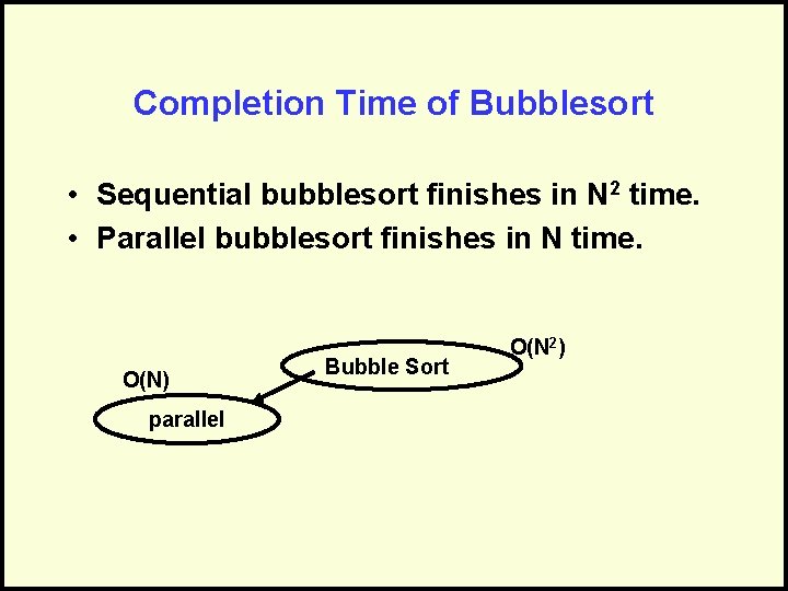
Completion Time of Bubblesort • Sequential bubblesort finishes in N 2 time. • Parallel bubblesort finishes in N time. O(N) parallel Bubble Sort O(N 2)
Product Complexity • • Got done in O(N) time, better than O(N 2) Each time “chunk” does O(N) work There are N time chunks. Thus, the amount of work is still O(N 2) • Product complexity is the amount of work per “time chunk” multiplied by the number of “time chunks” – the total work done.
Ceiling of Improvement • Parallelization can reduce time, but it cannot reduce work. The product complexity cannot change or improve. • How much improvement can parallelization provide? – Given an O(NLog. N) algorithm and Log N processors, the algorithm will take at least O(? ) time. O(N) – Given an O(N 3) algorithm and N processors, the algorithm will take at least O(? ) O(N 2)time.
Number of Processors • Processors are limited by hardware. • Typically, the number of processors is a power of 2 • Usually: The number of processors is a constant factor, 2 K • Conceivably: Networked computers joined as needed (ala Borg? ).
Adding Processors • A program on one processor – Runs in X time • Adding another processor – Runs in no more than X/2 time – Realistically, it will run in X/2 + time because of overhead • At some point, adding processors will not help and could degrade performance.
Overhead of Parallelization • Parallelization is not free. • Processors must be controlled and coordinated. • We need a way to govern which processor does what work; this involves extra work. • Often the program must be written in a special programming language for parallel systems. • Often, a parallelized program for one machine (with, say, 2 K processors) doesn’t work on other machines (with, say, 2 L processors).
What We Know about Tasks • Relatively isolated units of computation • Should be roughly equal in duration • Duration of the unit of work must be much greater than overhead time • Policy decisions and coordination required for shared data • Simpler algorithm are the easiest to parallelize

Questions?

More?
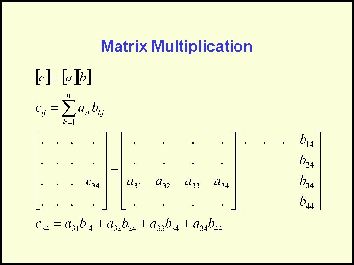
Matrix Multiplication
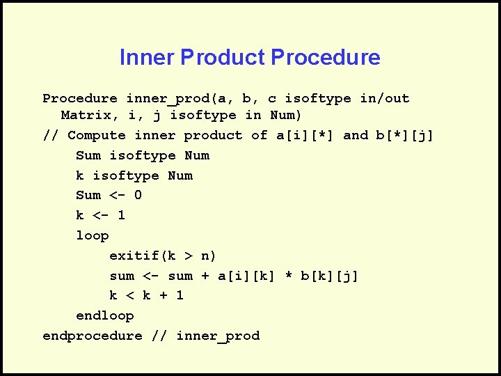
Inner Product Procedure inner_prod(a, b, c isoftype in/out Matrix, i, j isoftype in Num) // Compute inner product of a[i][*] and b[*][j] Sum isoftype Num k isoftype Num Sum <- 0 k <- 1 loop exitif(k > n) sum <- sum + a[i][k] * b[k][j] k < k + 1 endloop endprocedure // inner_prod
![Matrix definesa Array[1. . N] of Num N is // Declare constant defining size Matrix definesa Array[1. . N] of Num N is // Declare constant defining size](http://slidetodoc.com/presentation_image_h/a5e95c62e498187c886a2445d13e8068/image-101.jpg)
Matrix definesa Array[1. . N] of Num N is // Declare constant defining size // of arrays Algorithm P_Demo a, b, c isoftype Matrix Shared server isoftype Num Initialize(NUM_SERVERS) // Input a and b here // (code not shown) i, j isoftype Num
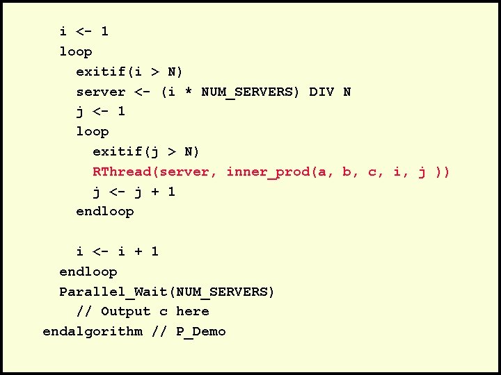
i <- 1 loop exitif(i > N) server <- (i * NUM_SERVERS) DIV N j <- 1 loop exitif(j > N) RThread(server, inner_prod(a, b, c, i, j )) j <- j + 1 endloop i <- i + 1 endloop Parallel_Wait(NUM_SERVERS) // Output c here endalgorithm // P_Demo

Questions?

- Slides: 104