B K Achille Stocchi LAL Orsay Universit Paris
 Achille Stocchi LAL Orsay Université")
( ν B � → K * γ ) Achille Stocchi LAL Orsay Université Paris Sud/IN 2 P 3 -CNRS 24 September 2008 DESY-Zeuthen M. Bona, M. Ciuchini, E. Franco, V. Lubicz, G. Martinelli, F. Parodi, M. Pierini, C. Schiavi, L. Silvestrini, A. Stocchi, V. Sordini, C. Tarantino and V. Vagnoni www. utfit. org Hints of New Physics in b→s transitions (or) Looking for New Physics in Flavour Physics in quark sector
 in")
~ half of the Standard Model Flavour Physics in the Standard Model (SM) in the quark sector: 10 free parameters 6 quarks masses 4 CKM parameters Wolfenstein parametrization : l , A, r, h h responsible of CP violation in SM In the Standard Model, charged weak interactions among quarks are codified in a 3 X 3 unitarity matrix : the CKM Matrix. The existence of this matrix conveys the fact that the quarks which participate to weak processes are a linear combination of mass eigenstates The fermion sector is poorly constrained by SM + Higgs Mechanism mass hierarchy and CKM parameters

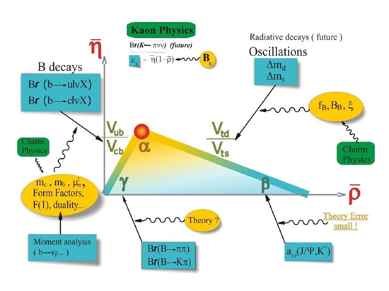
The Unitarity Triangle The CKM is unitary * + Vtd. V*tb = 0 * + Vcd. Vcb Vud. Vub 1 (b u)/(b c) md md/ ms +b+ = K b ρ2 Size of order l 3 : l 3 + η 2 ρ 2 + η 2 (1– ) ρ 2 + η 2 η [(1– ρ ) + P] f+, F(1), … f. B 2 d BBd ξ BK -

An example on how to fit the UT parameters and fit new physics b cℓ B and B: sdecays : 2/ B ccs : mixing /b B DK d. B / / 1 b uℓ K : CPV in K 3/
 function( , h…. ) Angles Sides + K")
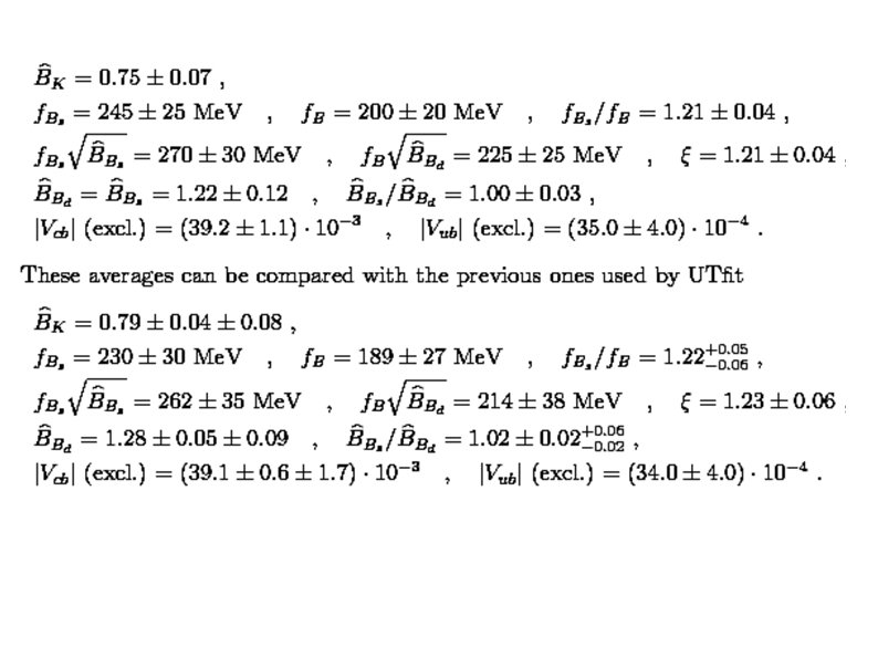
Fit with the Standard Model (SM) function( , h…. ) Angles Sides + K r = 0. 120 ± 0. 034 h = 0. 335 ± 0. 020 ρ = 0. 175 ± 0. 027 η = 0. 360 ± 0. 023

SM Fit Global Fit md, ms, Vub, Vcb, k + cos 2 b + a + g + 2 b+g Tremendous success of the CKM picture r = 0. 155 ± 0. 022 h = 0. 342 ± 0. 014

Should we stop here ? How to look for NP ? And in case of no observation to establish how much room is left for NP effects…? Long story… Some example in next 4 transparencies. .

some specific example of NP tests. . ms SM expectation Δms = (17. 5 ± 2. 1 ) ps-1 SM predictions of Dms LEP/SLD 1999 CDF 2006 LEP/SLD 2002 CDF only : signal at 5 s Δ ms = (17. 77 ± 0. 12) ps-1 Tevatron results Limited by Lattice calculations
o (up to π ambiguity)")
g Direct measurement From fit γ = (81 ± 13)o (up to π ambiguity) γ = (64. 0 ± 3. 0)o Summer 2007 Legenda agreement between the predicted values and the measurements at better than : 1 s 3 s 5 s 2 s 4 s 6 s Winter 2008 B factories results LHCb expected to contribute

sin 2 b vs Vub sin 2 b=0. 668 ± 0. 026 1. 5 s tension Vub(excl. ) =(35. 0± 4. 0)10 -4 Vub(incl. ) =(39. 9± 1. 5 ± 4. 0)10 -4 From fit sin 2 b=0. 736 ± 0. 034 Vub =(34. 8± 1. 6)10 -4 B factories results

Flavour Physics measure NP physics could be always arround the corner WHAT IS REALLY STRANGE IS THAT WE DID NOT SEE ANYTHING…. coupling Mass scale With masses of New Particles at few hundred Ge. V effects on measurable quantities should be important Problem known as the FLAVOUR PROBLEM Leff <~ 1 Te. V + flavour-mixing protected by additional symmetries (as MFV) Couplings can be still large if Leff > 1. . 10. . Te. V If there is NP at scale L, it will generate new operator of dimension D with coefficients proportional to L 4 -D d only operator of D=6 contribute. So that in fact you have a dependence on 1/ L 2

Today we concentrate on a Model Independent fit to DF=2 observable which show a 2. 5 s evidence of NP in the b s transitions

Fit in a NP model independent approach Parametrizing NP physics in DF=2 processes DF=2

Using the example of the Supersymmetry To help with a more specific example : Example for B oscillations (FCNC-DB=2) : dbd pr upper limit of the relative contribution of NP dbd NP physics coupling Leff NP scale (masses of new particles) If couplings ~ 1 dbq ~ 1 Leff ~ 10/ pr Te. V dbs ~1 Leff ~ 2/ pr Te. V all possible intermediate possibilities dbq ~ 0. 1 dbs ~0. 1 Leff ~ 1/ pr Te. V Leff ~ 0. 2/ pr Te. V Oversimplified picture : for a quantitative analysis see for instance Minimal Flavour Violation (couplings small as CKM elements) Leff ~ 0. 08/ pr Te. V UTfit collaboration JHEP 0803: 049, 2008 ar. Xiv: 0707. 0636

r, h Constraints Tree processes 1 3 family Cs js X X DGs/Gs X X Dms X ASL(Bs) X X Vub/Vcb X Dmd X ACP (J/Y K) X X ACP (D ( ), DK ) X X ASL X ~X K X 5 new free parameters Cs, js Bs mixing Cd, jd Bd mixing C K K mixing X X X ACP (J/Y ) C K X X ACH 1 2 familiy jd (DK) ( , , ) 2 3 family Cd X X Today : fit possible with 10 contraints and 7 free parameters (r, h, Cd, jd , Cs, js, C K)
o")
Bd CBd = 0. 96± 0. 23 Bd = -(2. 9 ± 1. 9)o ANP/ASM vs NP With present data ANP/ASM=0 @ 1. 5 s ANP/ASM ~1 only if NP~0 ANP/ASM ~0 -30% @95% prob. The sin 2 b tension produces a 1. 5 s effect on f(Bd) and the asymmetry in the Ad(NP)/Ad (SM) vs f(NP) plot

Bd Actual sensitivity for a generic NP phase in the Bd sector r=ANP/ASM~10 -15% This is not yet a prove that if NP should be MFV violating Just for showing the link between precision and mass scale r upper limit of the relative contribution of NP dbd NP physics coupling Leff NP scale (masses of new particles) Take a case where Leff ~ 80/ r Ge. V MORE PRECISION IS NEEDED Leff ~ (200 -250) Ge. V

Bs Bs sector : very recent results r, h Cd jd Cs js X X D 0, CDF (2006 -2007) t(Bs) , DGs/Gs X X CDF, D 0, LEP Dms X ASL(Bs) X ACH ACP (J/Y ) ~X CDF (~2006), D 0, LEP X D 0 (2007) X D 0, CDF (2007 -2008) The realm of Tevatron Vtd. Vcd + Vts. Vcs + Vtb. Vcb = 0 l 2 l 4 bs Recall that in Bd sector Vud. Vub + Vcd. Vcb + Vtd. Vtb = 0 l 3 l 3

s vs of DGs using Bs J/y Nota bene for the experimental result fs = -2 bs Angular (q, j , y) analysis as a function of the proper time. Similar to measurement of b in Bd J/y K*. Respect to the Bd case, there is additional sensitivity because of DGs term Dunietz, Fleisher and Nierste Phys. Re. V D 63: 114015, 2001 Experimentally q and j are well determined from the m from J/y y is the decay plane between the J/y and the .
")
Winter 2007 Before ICHEP 2008 with Bs J/y Not Bs J/y 3 s C(Bs) = 1. 11 ± 0. 32 (Bs) = (-69± 14)º U (-20± 14)º U (20± 5)º U (72± 8)º C(Bs)=1. 07± 0. 29 (Bs)=(-19. 9± 5. 6)o. U(-68. 2± 4. 9)º ar. Xiv: 0803. 0659 v 1 [hep-ph] 5 Mar 2008 SM

Bd 1 <--> 3 vs Bs 2 <--> 3 1 <--> 3 70% 10% ANPd/ASMd~0. 1 and ANPs/ASMs~0. 7 correspond to ANPd/ANPs~ l 2 i. e. to an additional l suppression.

After ICHEP 2008 -CKM 2008 ICHEP 2008. D 0 released the likelihood without assumptions on the strong phases C(Bs) = 0. 97 ± 0. 20 (Bs)=(-70 ± 7)o. U(-18 ± 7)o SM 3 s 2. 5 s New CDF data not included: new CDF likelihood “not ready yet” SM compatibility decreased in the CDF analysis
, Lars Sonnenschein")
Here the results from HFAG. Without additional constraints See Diego Tonello (CDF), Lars Sonnenschein (D 0) CKM 08 Rome

This result, if confirmed, will imply : - of course NP physics - NP not Minimal Flavour Violation (large couplings. . new particles not necessary below the Te. V scale - NP model must explain why effects on Bd (which can still be as large as 20%) and K systems are smaller 1 <-> 2: strong suppression 1 <-> 3: ≤ O(10%) 2 <-> 3: O(1) this pattern is not unexpected in flavour models and in SUSY-GUTs ge a p xt e ne Flavour physics central - Bd sector, for F=2 but also F=1 b s transitions - K sector - of course Bs sector Se PRECISION IS NEEDED
 Wb t B")
DF=1 b s transitions are very sensitive to NP contributions (DF=1) Wb t B 0 d d s s s d K 0 ~ g b ~ s s S(f. K) New Physics contribution (2 -3 families) The disagreement is much reduced PRECISION IS NEEDED CFMS B factories results Super. B expected to contribute Im(d 23)LR

- D 0 and CDF will update their results. They have not used entire dataset. If the NP phase stay so large they could observe it with the full/final dataset - js is a golden measurement for LHCb Simulation done with 4 fb-1. φBs = (0. 0 ± 1. 3)o CBs = 0. 99 ± 0. 12 But also with much less data, LHCb can observe the effect if will stay so large New studies show that (end 2009 ? ) LHCb with 0. 5 fb-1 s(f. Bs) = 0. 06 ATLAS with 2. 5 fb-1 s(f. Bs) = 0. 16 See Gaia Lanfranchi CKM 08/Rome

Flavour physics in the quark sector is in his mature age In b d transitions NP effect are “confined” to be at order less ~10 -15% ! New data from Tevatron show ~2. 5 s discrepancy from SM in b s transitions If confirmed would implies NP and not Minimal Flavour Violation Tevatron (with full statistics) and LHCb will clarify the discrepancy Flavour Physics is alive more than ever to look for NP beyond SM Super. B

BACKUP MATERIAL
=(1. 73± 0. 34)10 -4 B factories results")
B → tn Belle BR(B tu)=(1. 73± 0. 34)10 -4 B factories results Super. B expected to contribute

The problem of particle physics today is : where is the NP scale L ~ 0. 5, 1… 1016 Te. V The quantum stabilization of the Electroweak Scale suggest that L ~ 1 Te. V LHC will search on this range What happens if the NP scale is at 2 -3. . 10 Te. V …naturalness is not at loss yet… Flavour Physics explore also this range We want to perform flavour measurements such that : - if NP particles are discovered at LHC we able study the flavour structure of the NP - we can explore NP scale beyond the LHC reach If there is NP at scale L, it will generate new operator of dimension D with coefficients proportional to L 4 -D You could demonstrate that only operator of D=6 contribute So that in fact you have a dependence on 1/ L 2

Kaon sector

Flavour specific final states

Tagging is important to separate the time evolution of mesons produced as Bs or anti-Bs. In this way we obtain direct sensitivity to CP-violating phase. This phase enters with terms proportional to cos(2 bs) and sin(2 bs). Analyses which do not use flavour tagging are sensitive to |cos(2 bs)| and |sin(2 bs)|, leading to a four-fold ambiguities in the determination of js. Only two-fold ambiguity Te. Vatron results LHCb expected to contribute

1. 35 fb-1 2. 8 fb-1 Before ICHEP 2008 CDF tagged measurement D 0 tagged measurement Other measurements t. Bs, DG/G, ASL, ACH directly from the Likelihood given by CDF No likelihood available from D 0 Conservative approach used (for details see appendix) All available measured used with and up-to-date hadronic parameters Notice that the two measurements are in agreement Other measurements are also important
 D 0 data Strong phase taken also From Bd")
Modeling D 0 data (I) D 0 data Strong phase taken also From Bd J/y K* + SU(3) NO AMBIGUITY Used by UTFit The problem is that the singlet Component of the f is ignored. WE REINTRODUCE THE AMBIGUITY (mirroring the likelihood)

- Stability of the result, who is contributing more ? - Is an evidence…. How many sigmas ? Without tagged analyses D 0 and CDF Including only D 0 Gaussian Including only D 0 likelihood profile Depending of the approach used (for treating D 0 data) js is away from zero from 3 s up to 3. 7 s.
 DEFAULT METHOD We have the results with 7 x")
Modeling D 0 data (II) DEFAULT METHOD We have the results with 7 x 7 correlation matrix. Fit at 7 parameters we extract 2 parameters (DGs and js). Two others approach used to include non-Gaussian tails: -Scale errors such they agree with the quoted “ 2 s” ranges -Use the 1 D profile likelihood given by D 0 (fig 2).

ICHEP 2008. D 0 released the likelihood without assumption on the strong phases Move from 1. 35 fb-1 2. 8 fb-1

Evolution of this result The two most probable peaks of last summer are now enhanced

Looking at the result with a different parametrization js ~ -70 o Solution corresponding to js ~ -20 o As. NP / As. SM= (0. 73 ± 0. 35) js. NP = (-51 ± 11)o
- Slides: 42