Autonomous Mobile Robots Localization Position Global Map Environment

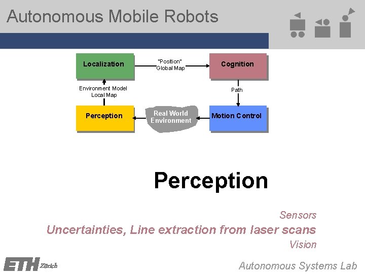
Autonomous Mobile Robots Localization "Position" Global Map Environment Model Local Map Perception Cognition Path Real World Environment Motion Control Perception Sensors Uncertainties, Line extraction from laser scans Vision Zürich Autonomous Systems Lab

4 b - Perception - Uncertainty 4 b 2 Perception – Uncertainty, Fusion § 4 a - Sensors § case studies § classification, performance § technology overview § 4 b – Uncertainties, Line extraction from laser scans § 4 c - Vision © R. Siegwart, D. Scaramuzza, ETH Zurich - ASL

4 b - Perception - Uncertainty 4 b 3 Uncertainty Representation § Sensing is always related to uncertainties. § § How can uncertainty be represented or quantified? How do they propagate - uncertainty of a function of uncertain values? How do uncertainties combine if different sensor reading are fused? What is the merit of all this for mobile robotics? © R. Siegwart, D. Scaramuzza, ETH Zurich - ASL

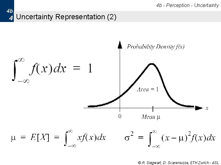
4 b - Perception - Uncertainty 4 b 4 Uncertainty Representation (2) © R. Siegwart, D. Scaramuzza, ETH Zurich - ASL

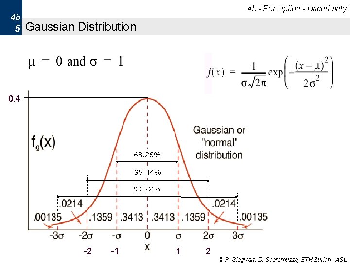
4 b - Perception - Uncertainty 4 b 5 Gaussian Distribution 0. 4 68. 26% 95. 44% 99. 72% -2 -1 1 2 © R. Siegwart, D. Scaramuzza, ETH Zurich - ASL

4 b - Perception - Uncertainty 4 b 6 The Error Propagation Law: Motivation § Imagine extracting a line based on point measurements with uncertainties. § The model parameters ri (length of the perpendicular) and qi (its angle to the abscissa) describe a line uniquely. § The question: § What is the uncertainty of the extracted line knowing the uncertainties of the measurement points that contribute to it ? © R. Siegwart, D. Scaramuzza, ETH Zurich - ASL

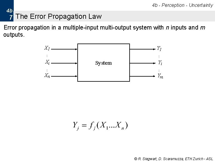
4 b - Perception - Uncertainty 4 b 7 The Error Propagation Law Error propagation in a multiple-input multi-output system with n inputs and m outputs. X 1 Xn System Yi … … Xi … … Y 1 Ym © R. Siegwart, D. Scaramuzza, ETH Zurich - ASL

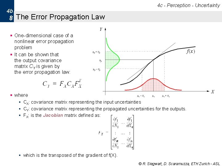
4 c - Perception - Uncertainty 4 b 8 The Error Propagation Law § One-dimensional case of a nonlinear error propagation problem § It can be shown that the output covariance matrix CY is given by the error propagation law: § where § CX: covariance matrix representing the input uncertainties § CY: covariance matrix representing the propagated uncertainties for the outputs. § FX: is the Jacobian matrix defined as: § which is the transposed of the gradient of f(X). © R. Siegwart, D. Scaramuzza, ETH Zurich - ASL

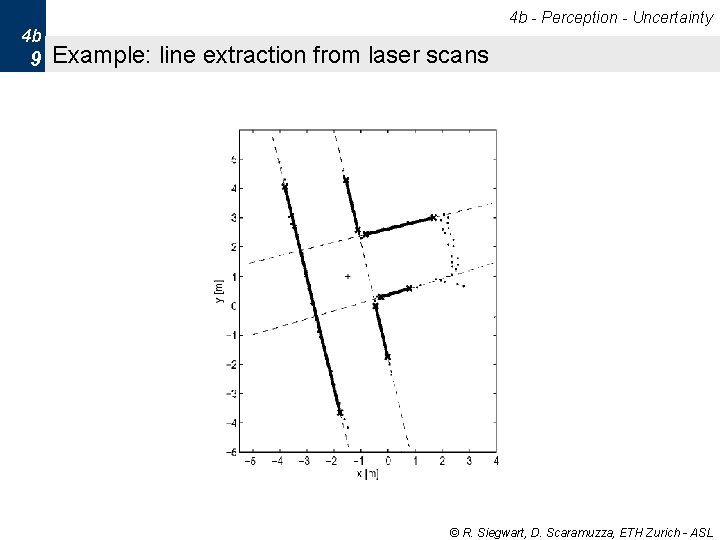
4 b - Perception - Uncertainty 4 b 9 Example: line extraction from laser scans © R. Siegwart, D. Scaramuzza, ETH Zurich - ASL

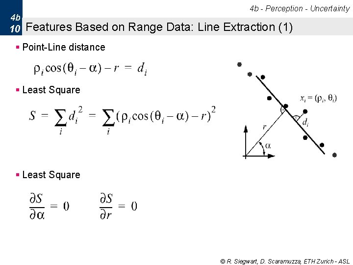
4 b - Perception - Uncertainty 4 b 10 Features Based on Range Data: Line Extraction (1) § Point-Line distance § Least Square © R. Siegwart, D. Scaramuzza, ETH Zurich - ASL

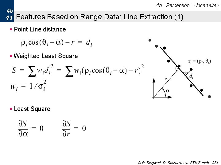
4 b - Perception - Uncertainty 4 b 11 Features Based on Range Data: Line Extraction (1) § Point-Line distance § Weighted Least Square § Least Square © R. Siegwart, D. Scaramuzza, ETH Zurich - ASL

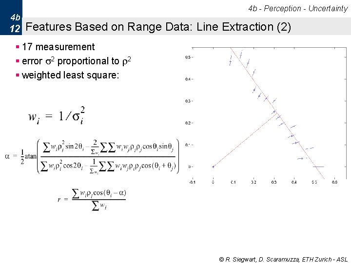
4 b - Perception - Uncertainty 4 b 12 Features Based on Range Data: Line Extraction (2) § 17 measurement § error s 2 proportional to r 2 § weighted least square: © R. Siegwart, D. Scaramuzza, ETH Zurich - ASL

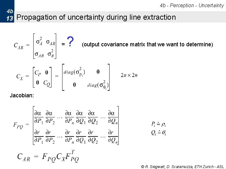
4 b - Perception - Uncertainty 4 b 13 Propagation of uncertainty during line extraction = ? (output covariance matrix that we want to determine) Jacobian: © R. Siegwart, D. Scaramuzza, ETH Zurich - ASL

Autonomous Mobile Robots Line & Plane Features Zürich Autonomous Systems Lab

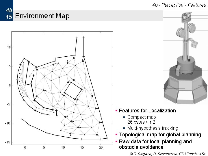
4 b - Perception - Features 4 b 15 Environment Map § Features for Localization § Compact map 26 bytes / m 2 § Multi-hypothesis tracking § Topological map for global planning § Raw data for local planning and obstacle avoidance © R. Siegwart, D. Scaramuzza, ETH Zurich - ASL

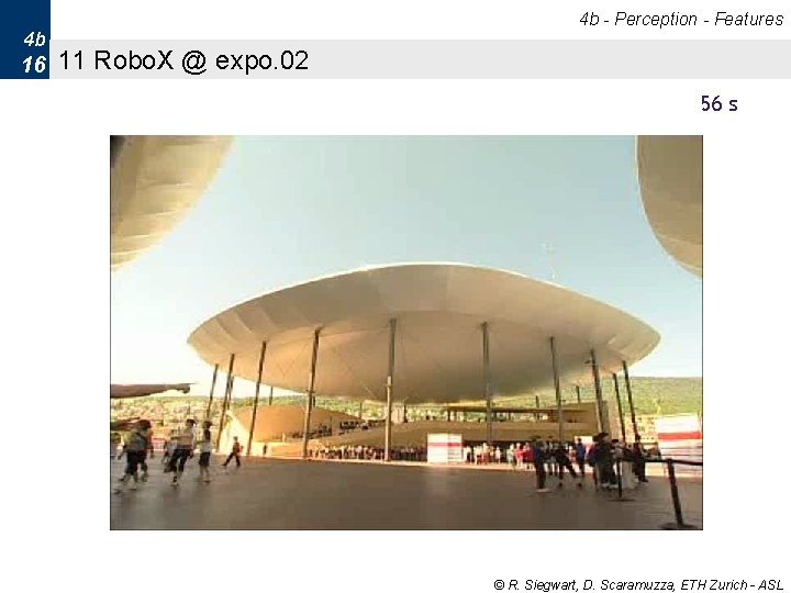
4 b - Perception - Features 4 b 16 11 Robo. X @ expo. 02 56 s © R. Siegwart, D. Scaramuzza, ETH Zurich - ASL

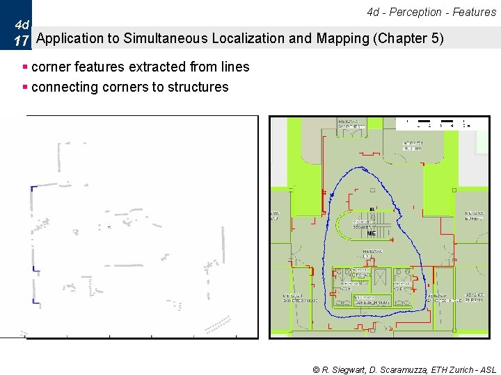
4 d - Perception - Features 4 d 17 Application to Simultaneous Localization and Mapping (Chapter 5) § corner features extracted from lines § connecting corners to structures © R. Siegwart, D. Scaramuzza, ETH Zurich - ASL

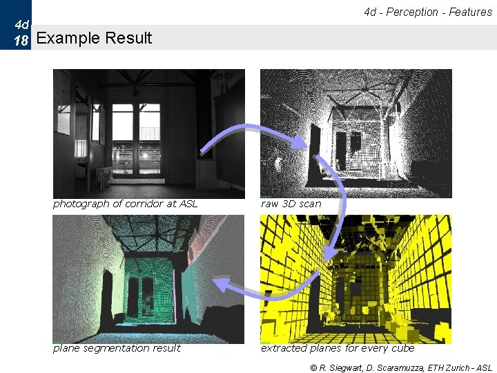
4 d - Perception - Features 4 d 18 Example Result photograph of corridor at ASL raw 3 D scan plane segmentation result extracted planes for every cube © R. Siegwart, D. Scaramuzza, ETH Zurich - ASL

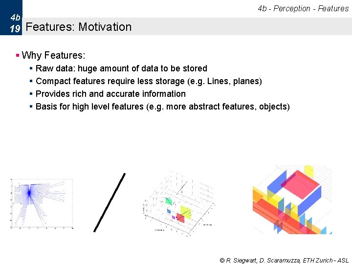
4 b - Perception - Features 4 b 19 Features: Motivation § Why Features: § § Raw data: huge amount of data to be stored Compact features require less storage (e. g. Lines, planes) Provides rich and accurate information Basis for high level features (e. g. more abstract features, objects) © R. Siegwart, D. Scaramuzza, ETH Zurich - ASL

Autonomous Mobile Robots Line Extraction Split and merge Linear regression RANSAC Hough-Transform Zürich Autonomous Systems Lab

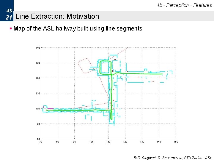
4 b - Perception - Features 4 b 21 Line Extraction: Motivation § Map of the ASL hallway built using line segments © R. Siegwart, D. Scaramuzza, ETH Zurich - ASL

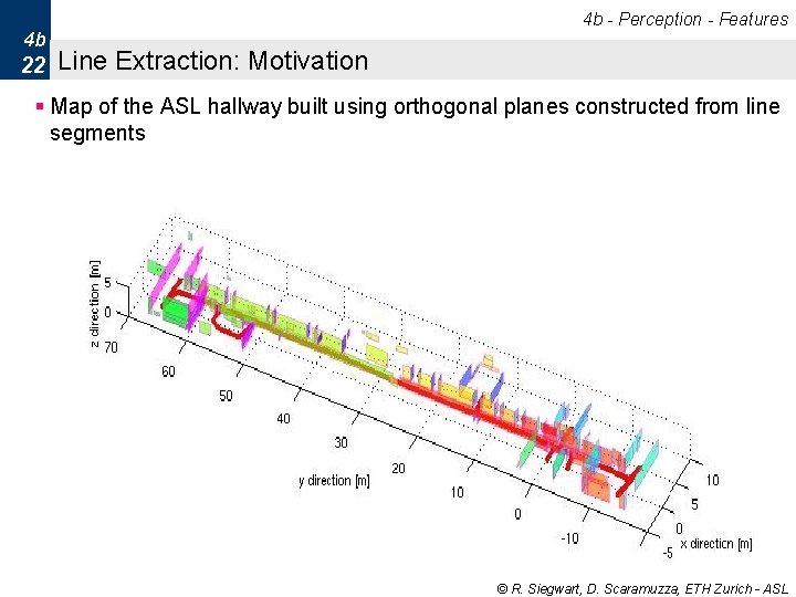
4 b - Perception - Features 4 b 22 Line Extraction: Motivation § Map of the ASL hallway built using orthogonal planes constructed from line segments © R. Siegwart, D. Scaramuzza, ETH Zurich - ASL

4 b - Perception - Features 4 b 23 Line Extraction: Motivation § Why laser scanner: § Dense and accurate range measurements § High sampling rate, high angular resolution § Good range distance and resolution. § Why line segment: § § The simplest geometric primitive Compact, requires less storage Provides rich and accurate information Represents most office-like environment. © R. Siegwart, D. Scaramuzza, ETH Zurich - ASL

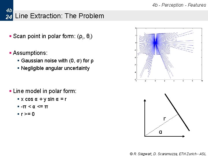
4 b - Perception - Features 4 b 24 Line Extraction: The Problem § Scan point in polar form: (ρi, θi) § Assumptions: § Gaussian noise with (0, σ) for ρ § Negligible angular uncertainty § Line model in polar form: § x cos α + y sin α = r § -π < α <= π § r >= 0 r α © R. Siegwart, D. Scaramuzza, ETH Zurich - ASL

4 b - Perception - Features 4 b 25 Line Extraction: The Problem (2) § Three main problems: § How many lines ? § Which points belong to which line ? • This problem is called SEGMENTATION § Given points that belong to a line, how to estimate the line parameters ? • This problem is called LINE FITTING § The Algorithms we will see: 1. 2. 3. 4. Split and merge Linear regression RANSAC Hough-Transform © R. Siegwart, D. Scaramuzza, ETH Zurich - ASL

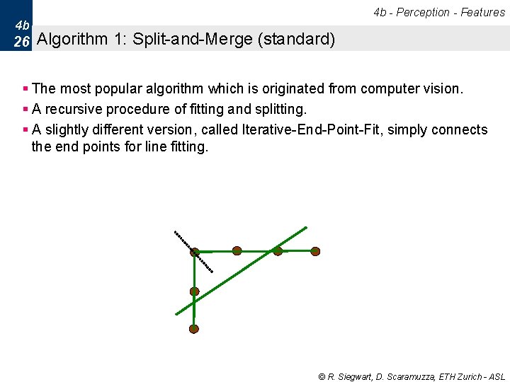
4 b - Perception - Features 4 b 26 Algorithm 1: Split-and-Merge (standard) § The most popular algorithm which is originated from computer vision. § A recursive procedure of fitting and splitting. § A slightly different version, called Iterative-End-Point-Fit, simply connects the end points for line fitting. © R. Siegwart, D. Scaramuzza, ETH Zurich - ASL

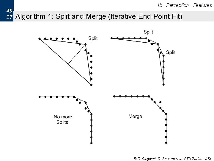
4 b - Perception - Features 4 b 27 Algorithm 1: Split-and-Merge (Iterative-End-Point-Fit) © R. Siegwart, D. Scaramuzza, ETH Zurich - ASL

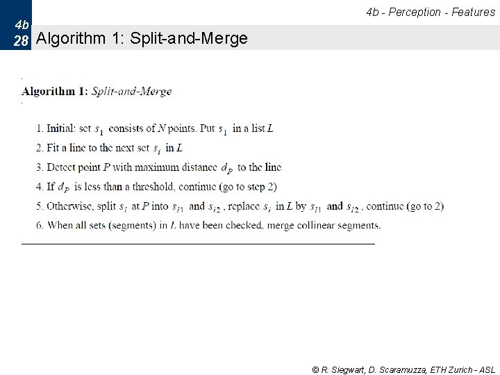
4 b - Perception - Features 4 b 28 Algorithm 1: Split-and-Merge © R. Siegwart, D. Scaramuzza, ETH Zurich - ASL

4 b - Perception - Features 4 b 29 Algorithm 1: Split-and-Merge: Example application © R. Siegwart, D. Scaramuzza, ETH Zurich - ASL

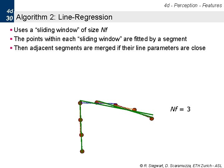
4 d - Perception - Features 4 d 30 Algorithm 2: Line-Regression § Uses a “sliding window” of size Nf § The points within each “sliding window” are fitted by a segment § Then adjacent segments are merged if their line parameters are close Nf = 3 © R. Siegwart, D. Scaramuzza, ETH Zurich - ASL

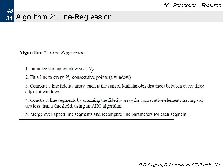
4 d - Perception - Features 4 d 31 Algorithm 2: Line-Regression © R. Siegwart, D. Scaramuzza, ETH Zurich - ASL

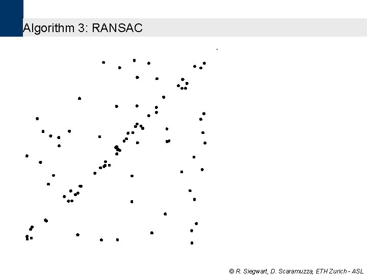
4 d - Perception - Features 4 d 32 Algorithm 3: RANSAC § Acronym of Random Sample Consensus. § It is a generic and robust fitting algorithm of models in the presence of outliers (points which do not satisfy a model) § RANSAC is not restricted to line extraction from laser data but it can be generally applied to any problem where the goal is to identify the inliers which satisfy a predefined mathematical model. § Typical applications in robotics are: line extraction from 2 D range data (sonar or laser); plane extraction from 3 D range data, and structure from motion § RANSAC is an iterative method and is non-deterministic in that the probability to find a line free of outliers increases as more iterations are used § Drawback: A nondeterministic method, results are different between runs. © R. Siegwart, D. Scaramuzza, ETH Zurich - ASL

Algorithm 3: RANSAC © R. Siegwart, D. Scaramuzza, ETH Zurich - ASL

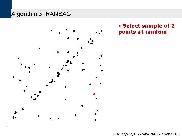
Algorithm 3: RANSAC • Select sample of 2 points at random © R. Siegwart, D. Scaramuzza, ETH Zurich - ASL

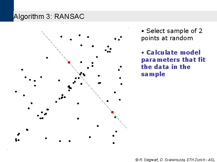
Algorithm 3: RANSAC • Select sample of 2 points at random • Calculate model parameters that fit the data in the sample © R. Siegwart, D. Scaramuzza, ETH Zurich - ASL

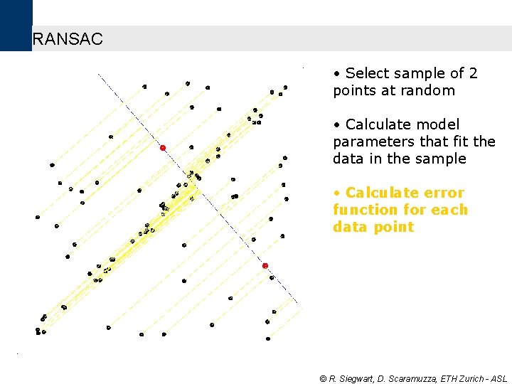
RANSAC • Select sample of 2 points at random • Calculate model parameters that fit the data in the sample • Calculate error function for each data point © R. Siegwart, D. Scaramuzza, ETH Zurich - ASL

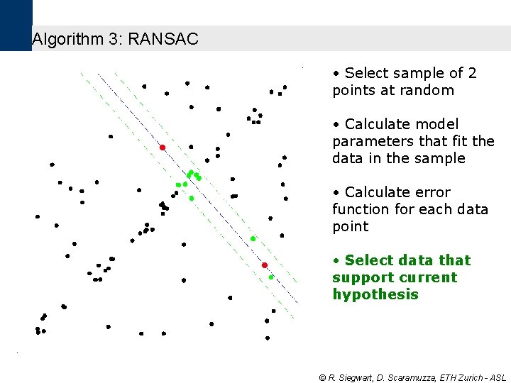
Algorithm 3: RANSAC • Select sample of 2 points at random • Calculate model parameters that fit the data in the sample • Calculate error function for each data point • Select data that support current hypothesis © R. Siegwart, D. Scaramuzza, ETH Zurich - ASL

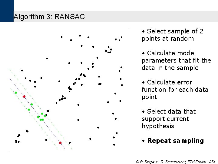
Algorithm 3: RANSAC • Select sample of 2 points at random • Calculate model parameters that fit the data in the sample • Calculate error function for each data point • Select data that support current hypothesis • Repeat sampling © R. Siegwart, D. Scaramuzza, ETH Zurich - ASL

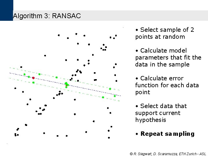
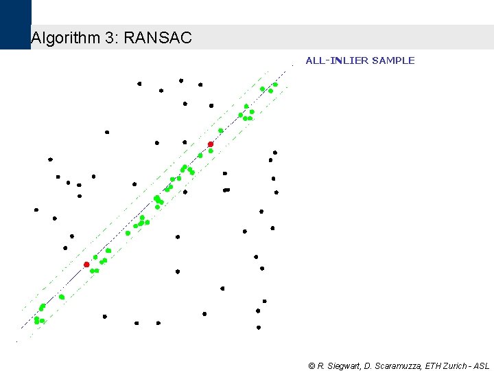
Algorithm 3: RANSAC ALL-INLIER SAMPLE © R. Siegwart, D. Scaramuzza, ETH Zurich - ASL

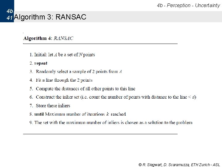
4 b - Perception - Uncertainty 4 b 41 Algorithm 3: RANSAC © R. Siegwart, D. Scaramuzza, ETH Zurich - ASL

4 b - Perception - Uncertainty 4 b 42 Algorithm 3: RANSAC How many iterations does RANSAC need? § Because we cannot know in advance if the observed set contains the maximum number of inliers, the ideal would be to check all possible combinations of 2 points in a dataset of N points. § The number of combinations is given by N(N-1)/2, which makes it computationally unfeasible if N is too large. For example, in a laser scan of 360 points we would need to check all 360*359/2= 64, 620 possibilities! § Do we really need to check all possibilities or can we stop RANSAC after iterations? The answer is that indeed we do not need to check all combinations but just a subset of them if we have a rough estimate of the percentage of inliers in our dataset § This can be done in a probabilistic way © R. Siegwart, D. Scaramuzza, ETH Zurich - ASL

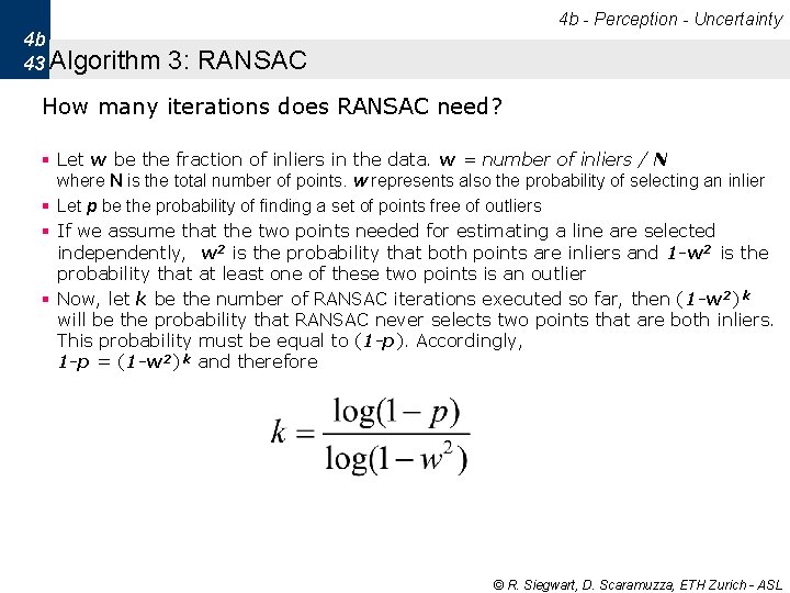
4 b - Perception - Uncertainty 4 b 43 Algorithm 3: RANSAC How many iterations does RANSAC need? § Let w be the fraction of inliers in the data. w = number of inliers / N where N is the total number of points. w represents also the probability of selecting an inlier § Let p be the probability of finding a set of points free of outliers § If we assume that the two points needed for estimating a line are selected independently, w 2 is the probability that both points are inliers and 1 -w 2 is the probability that at least one of these two points is an outlier § Now, let k be the number of RANSAC iterations executed so far, then (1 -w 2) k will be the probability that RANSAC never selects two points that are both inliers. This probability must be equal to (1 -p). Accordingly, 1 -p = (1 -w 2) k and therefore © R. Siegwart, D. Scaramuzza, ETH Zurich - ASL

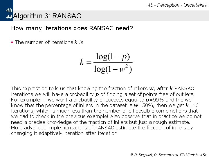
4 b - Perception - Uncertainty 4 b 44 Algorithm 3: RANSAC How many iterations does RANSAC need? § The number of iterations k is This expression tells us that knowing the fraction of inliers w, after k RANSAC iterations we will have a probability p of finding a set of points free of outliers. For example, if we want a probability of success equal to p=99% and the we know that the percentage of inliers in the dataset is w=50%, then we get k=16 iterations, which is much less than the number of all possible combinations that we had to check in the previous example! Also observe that in practice we do not need a precise knowledge of the fraction of inliers but just a rough estimate. More advanced implementations of RANSAC estimate the fraction of inliers by changing it adaptively iteration after iteration. © R. Siegwart, D. Scaramuzza, ETH Zurich - ASL

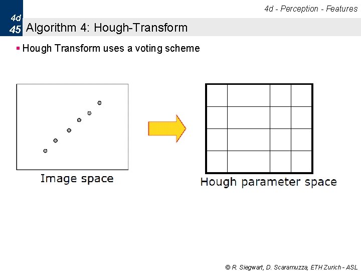
4 d - Perception - Features 4 d 45 Algorithm 4: Hough-Transform § Hough Transform uses a voting scheme © R. Siegwart, D. Scaramuzza, ETH Zurich - ASL

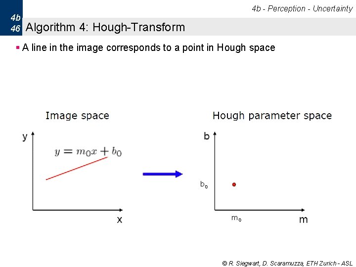
4 b - Perception - Uncertainty 4 b 46 Algorithm 4: Hough-Transform § A line in the image corresponds to a point in Hough space b 0 m 0 © R. Siegwart, D. Scaramuzza, ETH Zurich - ASL

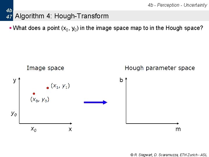
4 b - Perception - Uncertainty 4 b 47 Algorithm 4: Hough-Transform § What does a point (x 0, y 0) in the image space map to in the Hough space? © R. Siegwart, D. Scaramuzza, ETH Zurich - ASL

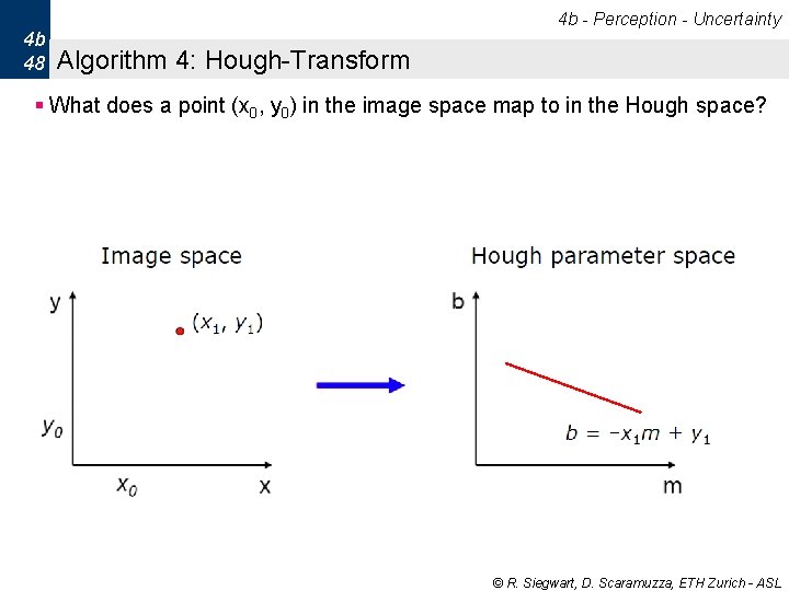
4 b - Perception - Uncertainty 4 b 48 Algorithm 4: Hough-Transform § What does a point (x 0, y 0) in the image space map to in the Hough space? © R. Siegwart, D. Scaramuzza, ETH Zurich - ASL

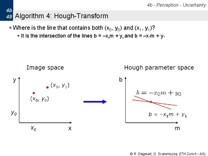
4 b - Perception - Uncertainty 4 b 49 Algorithm 4: Hough-Transform § Where is the line that contains both (x 0, y 0) and (x 1, y 1)? § It is the intersection of the lines b = –x m + y and b = –x 1 m + y 1 0 0 © R. Siegwart, D. Scaramuzza, ETH Zurich - ASL

4 b - Perception - Uncertainty 4 b 50 Algorithm 4: Hough-Transform § Problems with the (m, b) space: § Unbounded parameter domain § Vertical lines require infinite m © R. Siegwart, D. Scaramuzza, ETH Zurich - ASL

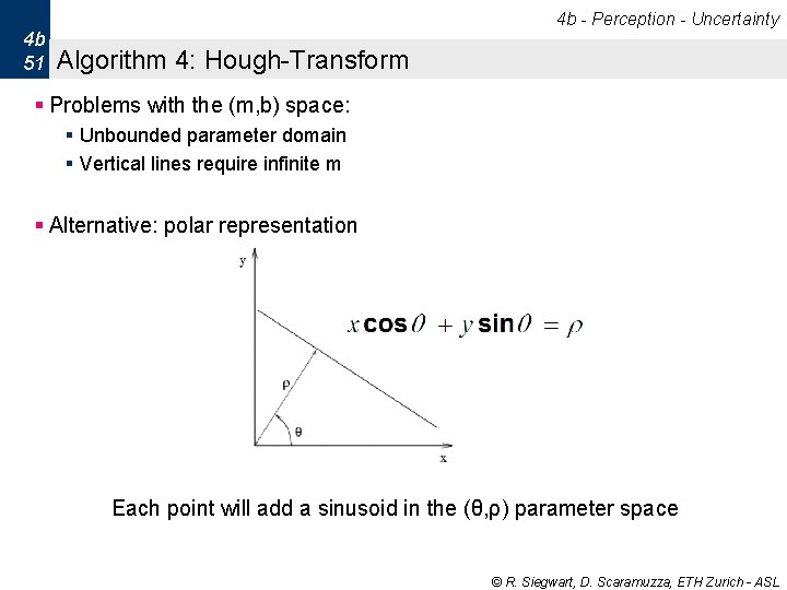
4 b - Perception - Uncertainty 4 b 51 Algorithm 4: Hough-Transform § Problems with the (m, b) space: § Unbounded parameter domain § Vertical lines require infinite m § Alternative: polar representation Each point will add a sinusoid in the (θ, ρ) parameter space © R. Siegwart, D. Scaramuzza, ETH Zurich - ASL

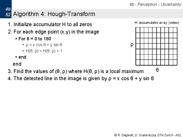
4 b - Perception - Uncertainty 4 b 52 Algorithm 4: Hough-Transform 1. Initialize accumulator H to all zeros 2. For each edge point (x, y) in the image § For θ = 0 to 180 • ρ = x cos θ + y sin θ • H(θ, ρ) = H(θ, ρ) + 1 § end 3. Find the values of (θ, ρ) where H(θ, ρ) is a local maximum 4. The detected line in the image is given by ρ = x cos θ + y sin θ © R. Siegwart, D. Scaramuzza, ETH Zurich - ASL

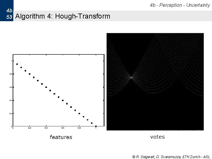
4 b - Perception - Uncertainty 4 b 53 Algorithm 4: Hough-Transform © R.

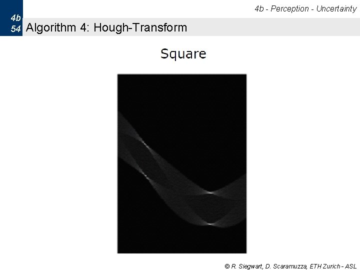
4 b - Perception - Uncertainty 4 b 54 Algorithm 4: Hough-Transform © R.

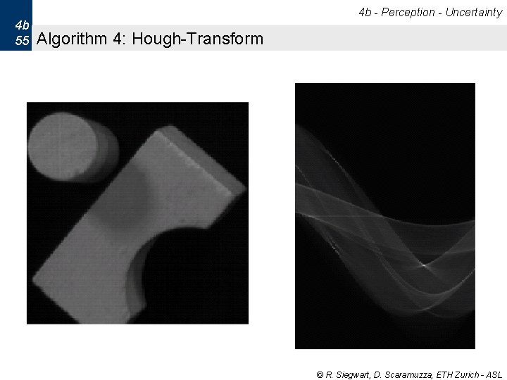
4 b - Perception - Uncertainty 4 b 55 Algorithm 4: Hough-Transform © R.

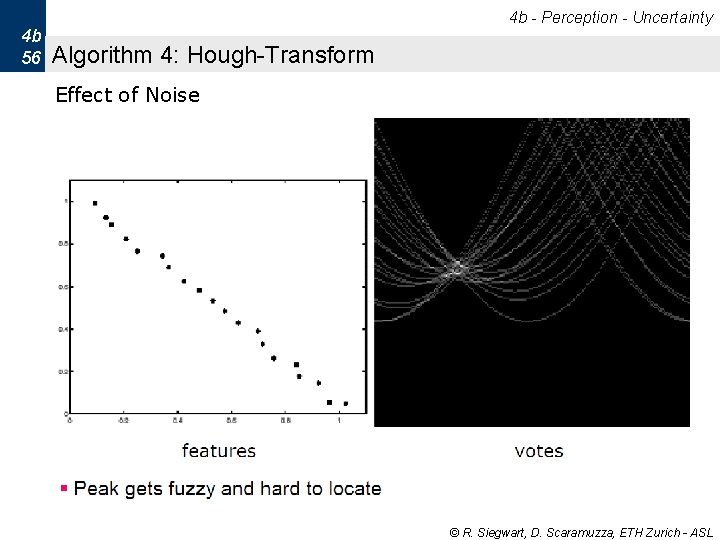
4 b - Perception - Uncertainty 4 b 56 Algorithm 4: Hough-Transform Effect of Noise © R. Siegwart, D. Scaramuzza, ETH Zurich - ASL

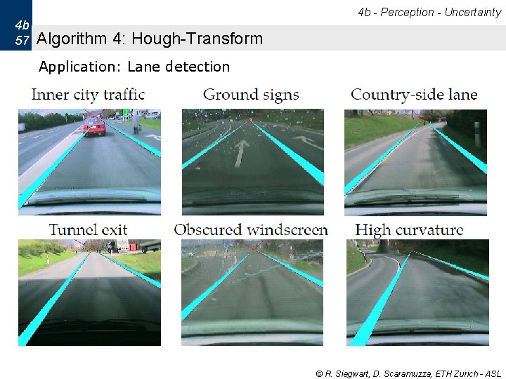
4 b - Perception - Uncertainty 4 b 57 Algorithm 4: Hough-Transform Application: Lane detection © R. Siegwart, D. Scaramuzza, ETH Zurich - ASL

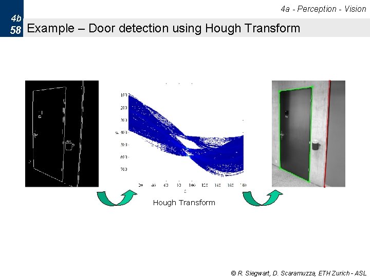
4 a - Perception - Vision 4 b 58 Example – Door detection using Hough Transform © R. Siegwart, D. Scaramuzza, ETH Zurich - ASL

4 d - Perception - Features 4 d 59 Comparison: Discussion § Deterministic methods perform better with laser scans § Split-and-merge, Line-Regression, Hough transform § Make use of the sequencing property of scan points. § Nondeterministic methods can produce high False. Pos § RANSAC § Do not use the sequencing property § But it can cope with outliers § Overall: § Split-and-merge is the fastest, best real-time applications © R. Siegwart, D. Scaramuzza, ETH Zurich - ASL

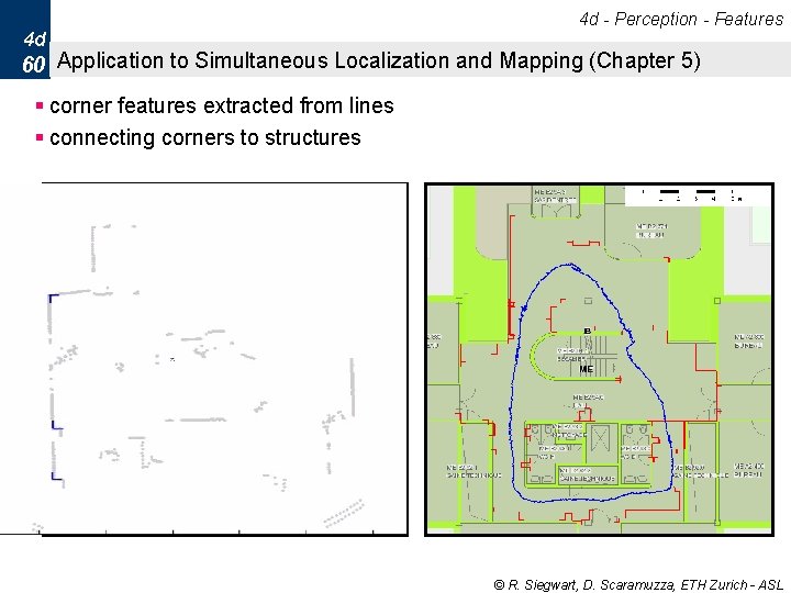
4 d - Perception - Features 4 d 60 Application to Simultaneous Localization and Mapping (Chapter 5) § corner features extracted from lines § connecting corners to structures © R. Siegwart, D. Scaramuzza, ETH Zurich - ASL

Autonomous Mobile Robots Plane Extraction Zürich Autonomous Systems Lab

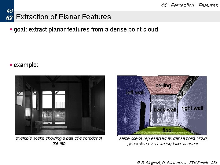
4 d - Perception - Features 4 d 62 Extraction of Planar Features § goal: extract planar features from a dense point cloud § example: ceiling left wall back wall right wall floor example scene showing a part of a corridor of the lab same scene represented as dense point cloud generated by a rotating laser scanner © R. Siegwart, D. Scaramuzza, ETH Zurich - ASL

4 d - Perception - Features 4 d 63 3 D Mapping § Laser Range Measurements aligned with ICP: § Six 3 D scans at 501*361 = 180’ 861 measurement points © R. Siegwart, D. Scaramuzza, ETH Zurich - ASL

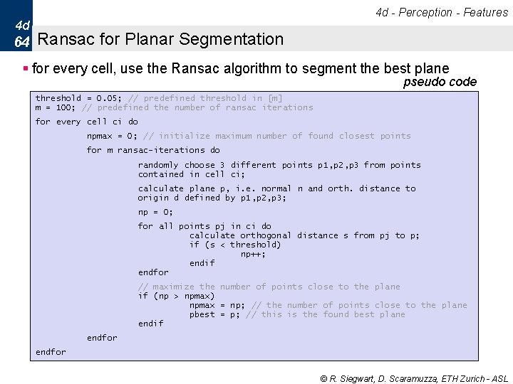
4 d - Perception - Features 4 d 64 Ransac for Planar Segmentation § for every cell, use the Ransac algorithm to segment the best plane pseudo code threshold = 0. 05; // predefined threshold in [m] m = 100; // predefined the number of ransac iterations for every cell ci do npmax = 0; // initialize maximum number of found closest points for m ransac-iterations do randomly choose 3 different points p 1, p 2, p 3 from points contained in cell ci; calculate plane p, i. e. normal n and orth. distance to origin d defined by p 1, p 2, p 3; np = 0; for all points pj in ci do calculate orthogonal distance s from pj to p; if (s < threshold) np++; endif endfor // maximize the number of points close to the plane if (np > npmax) npmax = np; // the number of points close to the plane pbest = p; // this is the found best plane endif endfor © R. Siegwart, D. Scaramuzza, ETH Zurich - ASL

4 d - Perception - Features 4 d 65 Example Result photograph of corridor at ASL raw 3 D scan plane segmentation result extracted planes for every cube © R. Siegwart, D. Scaramuzza, ETH Zurich - ASL

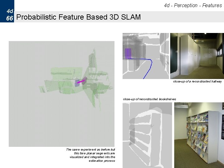
4 d - Perception - Features 4 d 66 Probabilistic Feature Based 3 D SLAM close-up of a reconstructed hallway close-up of reconstructed bookshelves The same experiment as before but this time planar segments are visualized and integrated into the estimation process © R. Siegwart, D. Scaramuzza, ETH Zurich - ASL

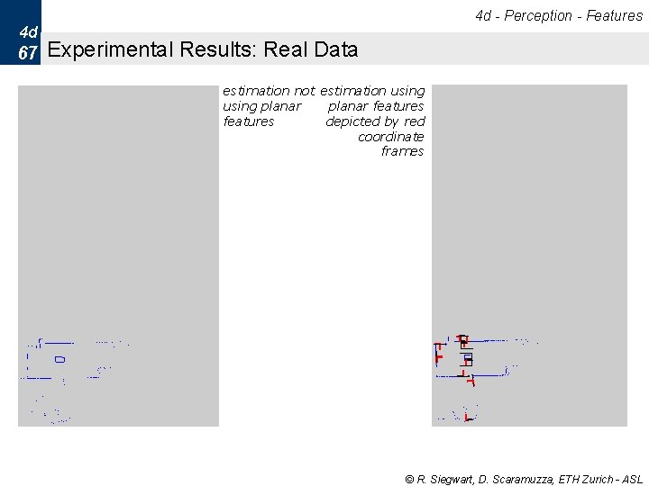
4 d - Perception - Features 4 d 67 Experimental Results: Real Data estimation not estimation using planar features depicted by red coordinate frames © R. Siegwart, D. Scaramuzza, ETH Zurich - ASL

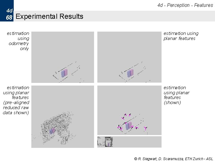
4 d - Perception - Features 4 d 68 Experimental Results estimation using odometry only estimation using planar features (pre-aligned reduced raw data shown) estimation using planar features (shown) © R. Siegwart, D. Scaramuzza, ETH Zurich - ASL

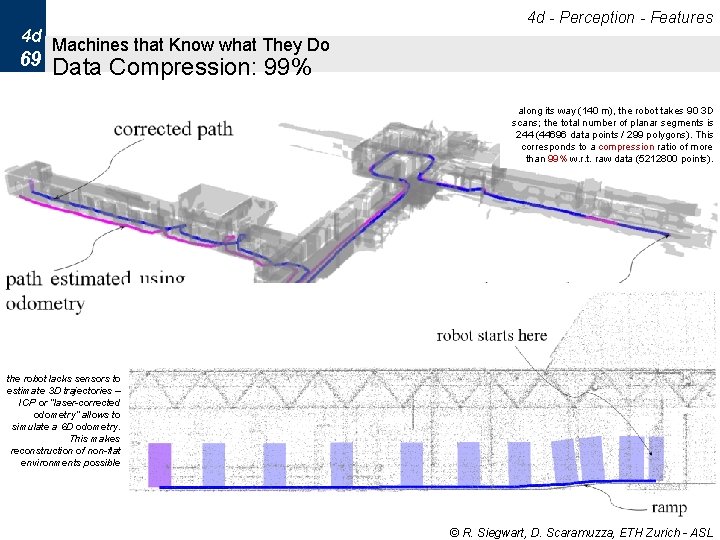
4 d - Perception - Features 4 d Machines that Know what They Do 69 Data Compression: 99% along its way (140 m), the robot takes 90 3 D scans; the total number of planar segments is 244 (44696 data points / 299 polygons). This corresponds to a compression ratio of more than 99% w. r. t. raw data (5212800 points). the robot lacks sensors to estimate 3 D trajectories – ICP or “laser-corrected odometry” allows to simulate a 6 D odometry. This makes reconstruction of non-flat environments possible © R. Siegwart, D. Scaramuzza, ETH Zurich - ASL