Autonomous CyberPhysical Systems Basics of Control Fall 2020

Autonomous Cyber-Physical Systems: Basics of Control Fall 2020. CS 513. Instructor: Jyo Deshmukh USC Viterbi School of Engineering Department of Computer Science

Layout Introduction to basics of linear control (without any Laplace transforms) Introduction to nonlinear control and rule-based control Introduction to observer design USC Viterbi School of Engineering Department of Computer Science 2

What is control theory? Engineering techniques and theory or control of dynamical systems Objective: Regulate system so that it behaves in desired fashion Ensure timely action to changes in system behavior Make sure control action does not cause system to … lose control Design challenge: Make a controller, scheduler, supervisor for the system to be controlled USC Viterbi School of Engineering Department of Computer Science 3

Open-loop vs. Closed-loop control Open-loop or feed-forward control Control action does not depend on plant output Most common form of control in many CPS applications! Pros: Cheaper, few sensors required, logic pretty straightforward Cons: Quality of control poor without human intervention Not adaptive! USC Viterbi School of Engineering Department of Computer Science 4 Controller Plant

Closed-loop or Feedback Controller adjusts controllable inputs in response to observed outputs Controller Can respond better to variations in disturbances Performance depends on how well outputs can be sensed, and how quickly controller can track changes in output Many different flavors of feedback control! USC Viterbi School of Engineering Department of Computer Science 5 Plant

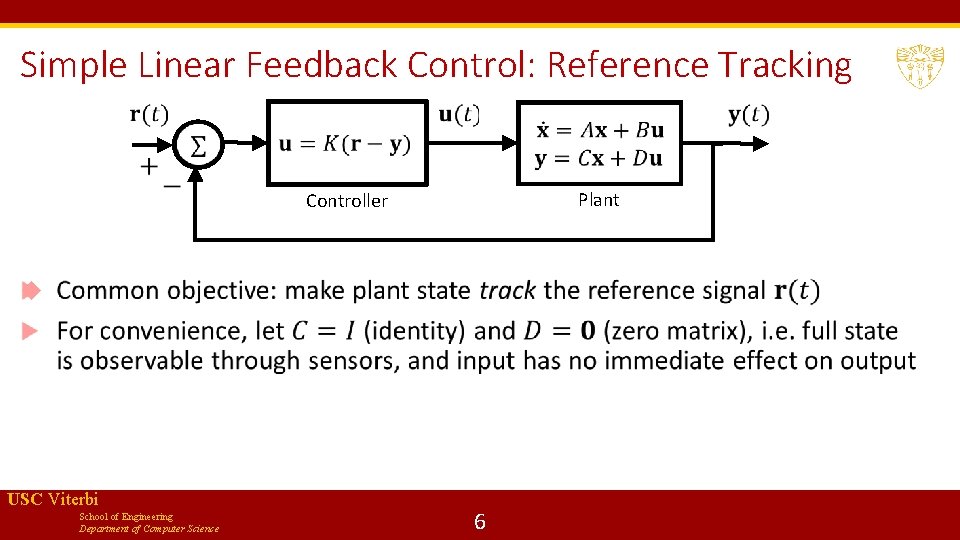
Simple Linear Feedback Control: Reference Tracking Plant Controller USC Viterbi School of Engineering Department of Computer Science 6

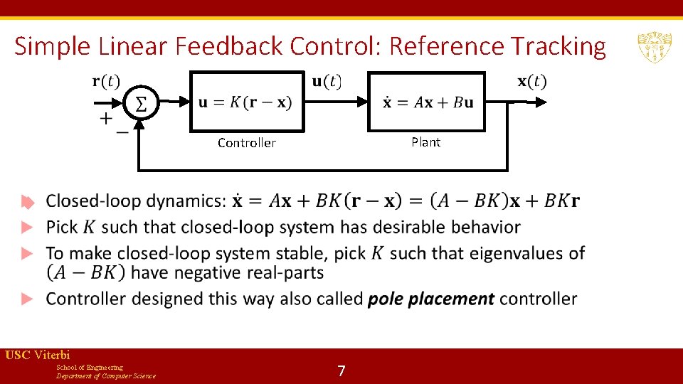
Simple Linear Feedback Control: Reference Tracking Plant Controller USC Viterbi School of Engineering Department of Computer Science 7

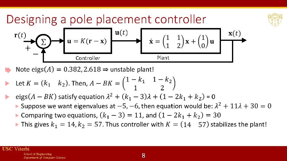
Designing a pole placement controller Plant Controller USC Viterbi School of Engineering Department of Computer Science 8

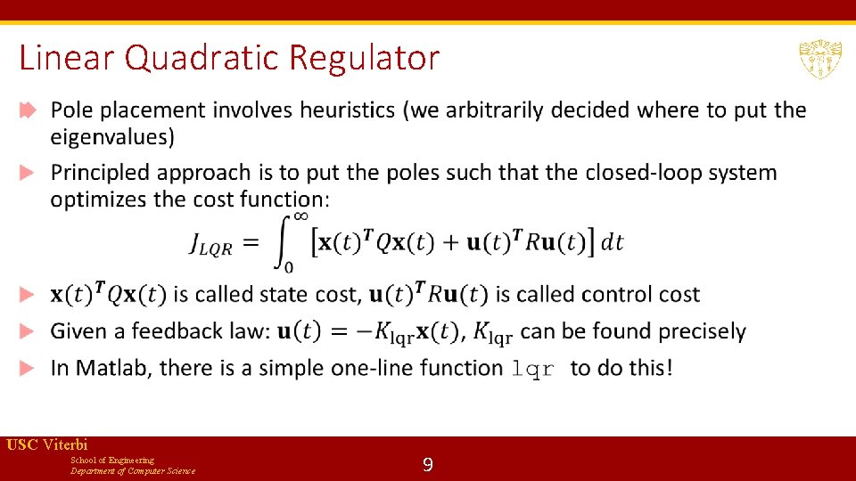
Linear Quadratic Regulator USC Viterbi School of Engineering Department of Computer Science 9

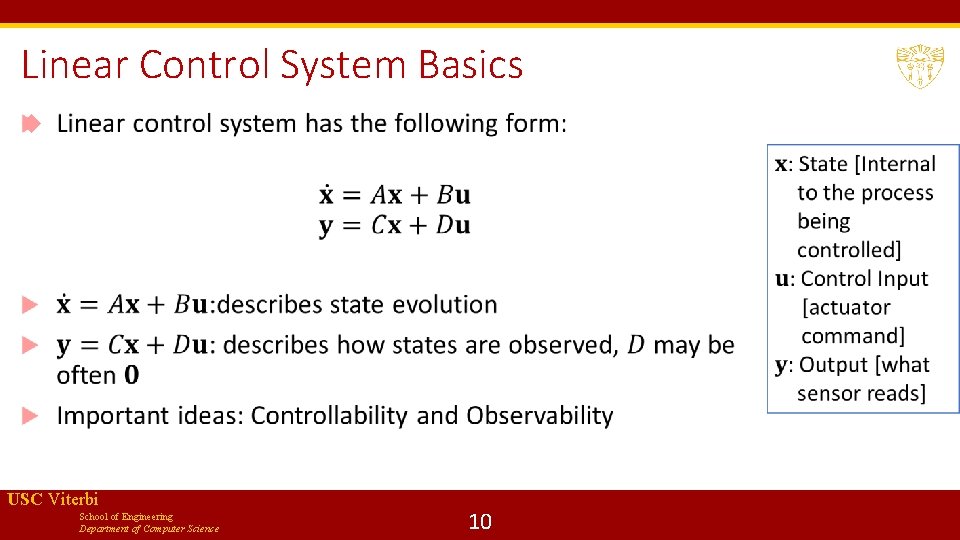
Linear Control System Basics USC Viterbi School of Engineering Department of Computer Science 10

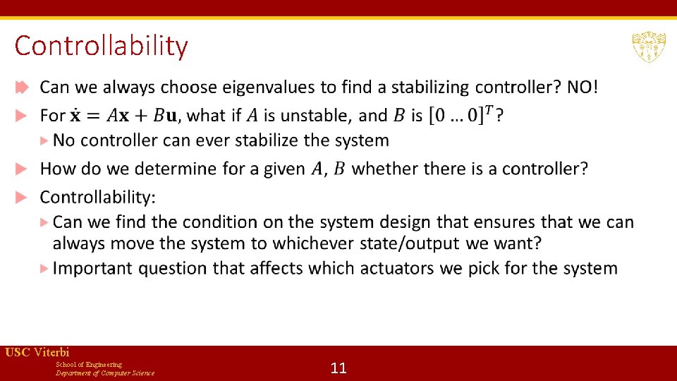
Controllability USC Viterbi School of Engineering Department of Computer Science 11

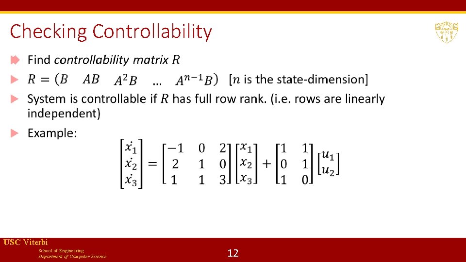
Checking Controllability USC Viterbi School of Engineering Department of Computer Science 12

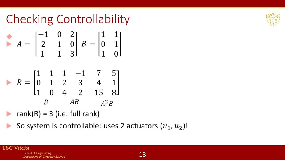
Checking Controllability USC Viterbi School of Engineering Department of Computer Science 13

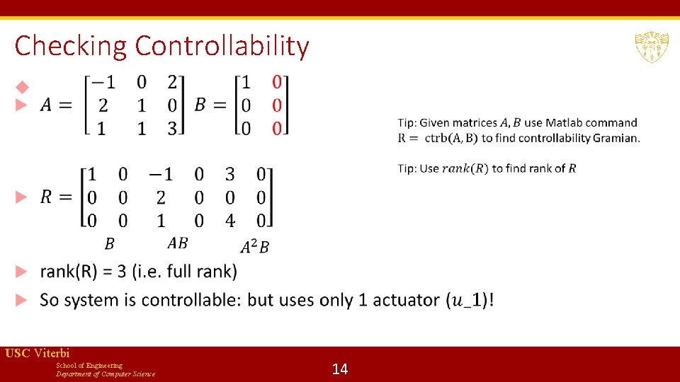
Checking Controllability USC Viterbi School of Engineering Department of Computer Science 14

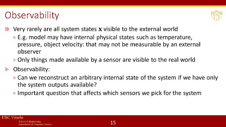
Observability USC Viterbi School of Engineering Department of Computer Science 15

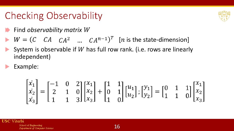
Checking Observability USC Viterbi School of Engineering Department of Computer Science 16

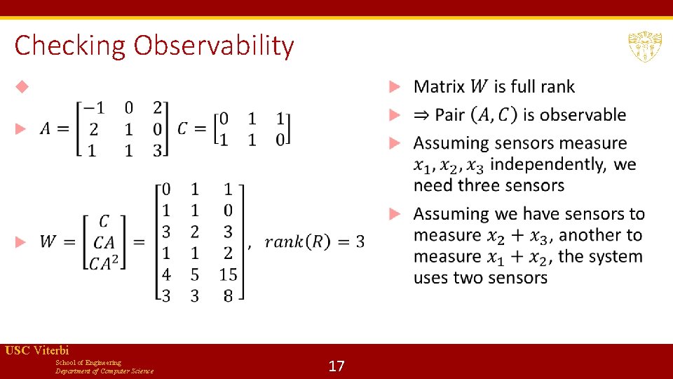
Checking Observability USC Viterbi School of Engineering Department of Computer Science 17

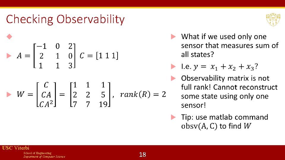
Checking Observability USC Viterbi School of Engineering Department of Computer Science 18

How do we reconstruct internal state? For linear systems (with no noise), this is done with the use of state estimators or observers For linear systems with noisy measurements and possible “process noise” in the system itself we use Kalman filter: introduced later in the course The most popular control method in the world started without any concerns of controllability, observability etc. Purpose: Tracking a given reference signal USC Viterbi School of Engineering Department of Computer Science 19

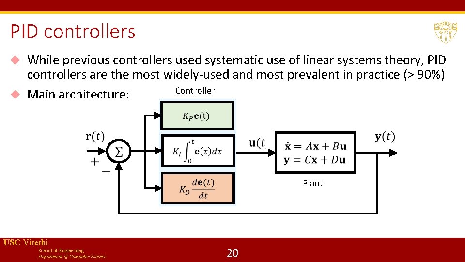
PID controllers While previous controllers used systematic use of linear systems theory, PID controllers are the most widely-used and most prevalent in practice (> 90%) Controller Main architecture: Plant USC Viterbi School of Engineering Department of Computer Science 20

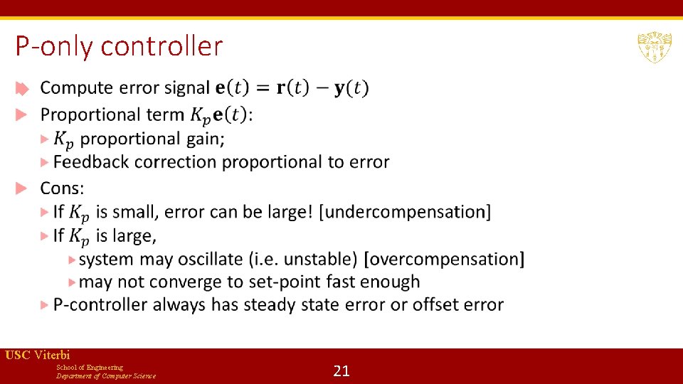
P-only controller USC Viterbi School of Engineering Department of Computer Science 21

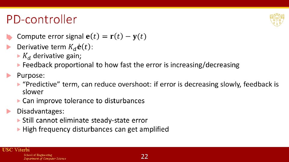
PD-controller USC Viterbi School of Engineering Department of Computer Science 22

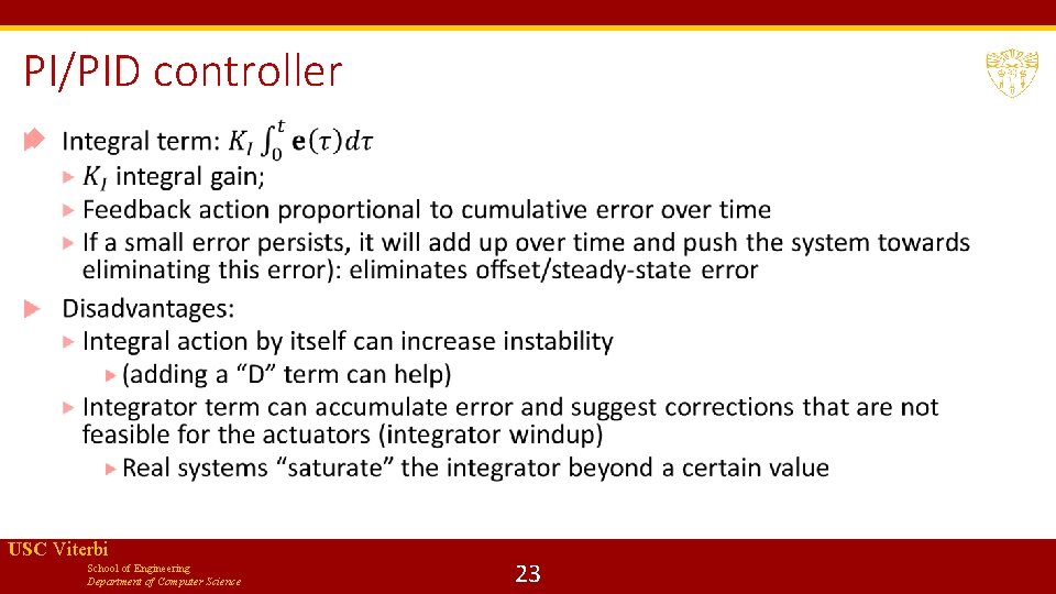
PI/PID controller USC Viterbi School of Engineering Department of Computer Science 23

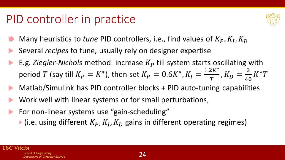
PID controller in practice USC Viterbi School of Engineering Department of Computer Science 24

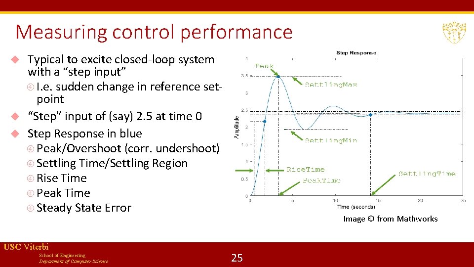
Measuring control performance Typical to excite closed-loop system with a “step input” I. e. sudden change in reference setpoint “Step” input of (say) 2. 5 at time 0 Step Response in blue Peak/Overshoot (corr. undershoot) Settling Time/Settling Region Rise Time Peak Time Steady State Error USC Viterbi School of Engineering Department of Computer Science Image © from Mathworks 25

Nonlinear Control USC Viterbi School of Engineering Department of Computer Science 26

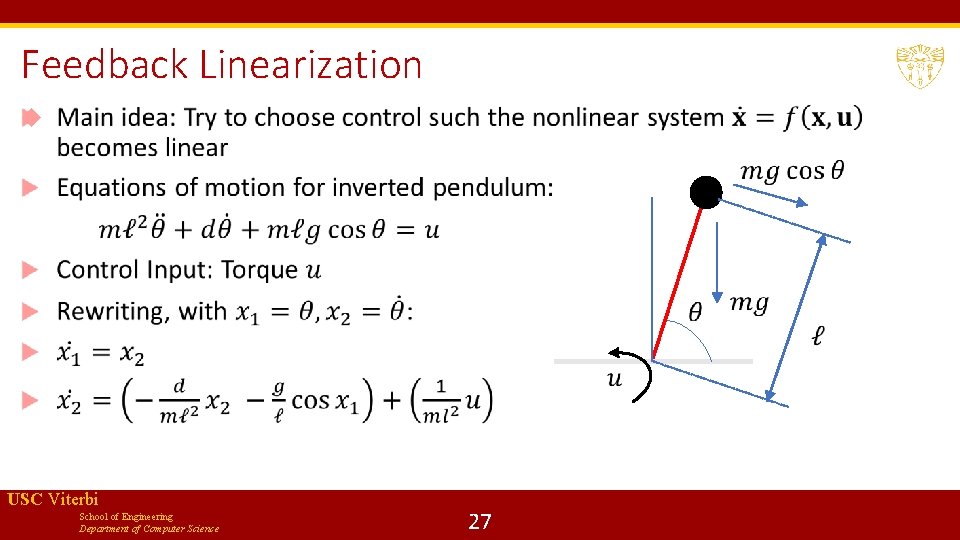
Feedback Linearization USC Viterbi School of Engineering Department of Computer Science 27

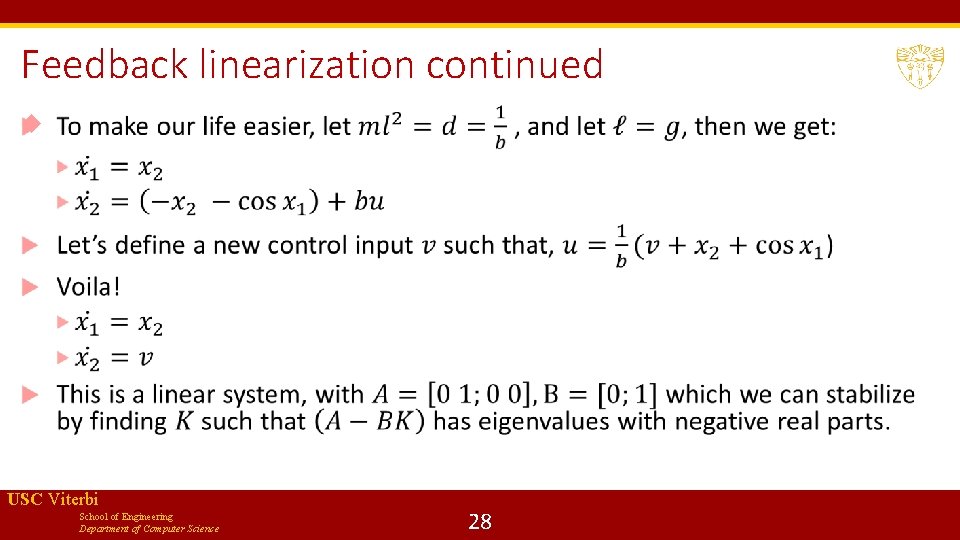
Feedback linearization continued USC Viterbi School of Engineering Department of Computer Science 28

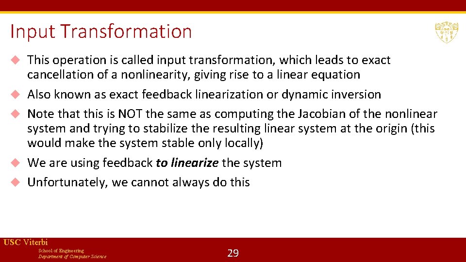
Input Transformation This operation is called input transformation, which leads to exact cancellation of a nonlinearity, giving rise to a linear equation Also known as exact feedback linearization or dynamic inversion Note that this is NOT the same as computing the Jacobian of the nonlinear system and trying to stabilize the resulting linear system at the origin (this would make the system stable only locally) We are using feedback to linearize the system Unfortunately, we cannot always do this USC Viterbi School of Engineering Department of Computer Science 29

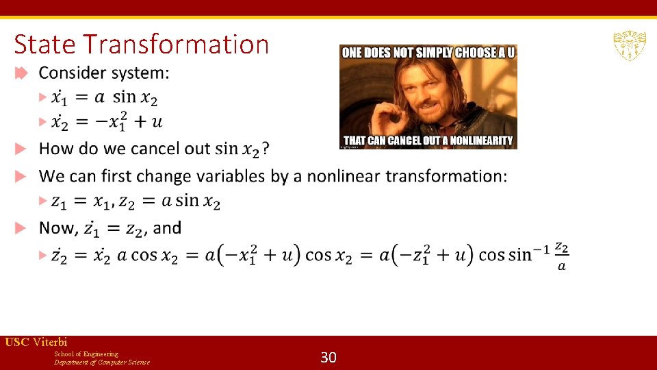
State Transformation USC Viterbi School of Engineering Department of Computer Science 30

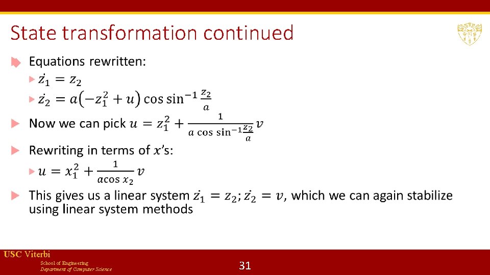
State transformation continued USC Viterbi School of Engineering Department of Computer Science 31

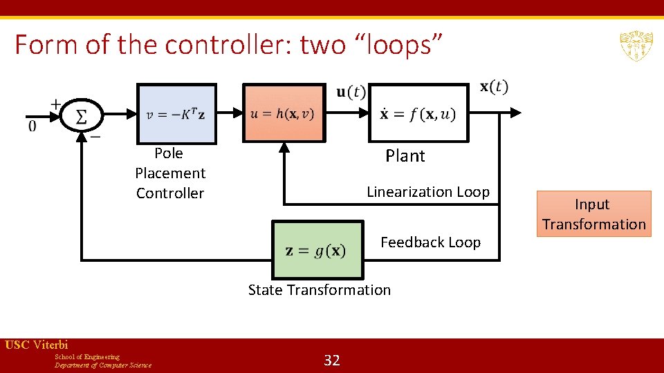
Form of the controller: two “loops” Pole Placement Controller Plant Linearization Loop Feedback Loop State Transformation USC Viterbi School of Engineering Department of Computer Science 32 Input Transformation

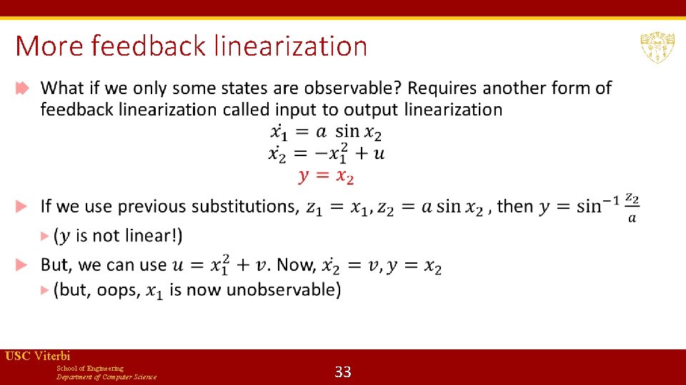
More feedback linearization USC Viterbi School of Engineering Department of Computer Science 33

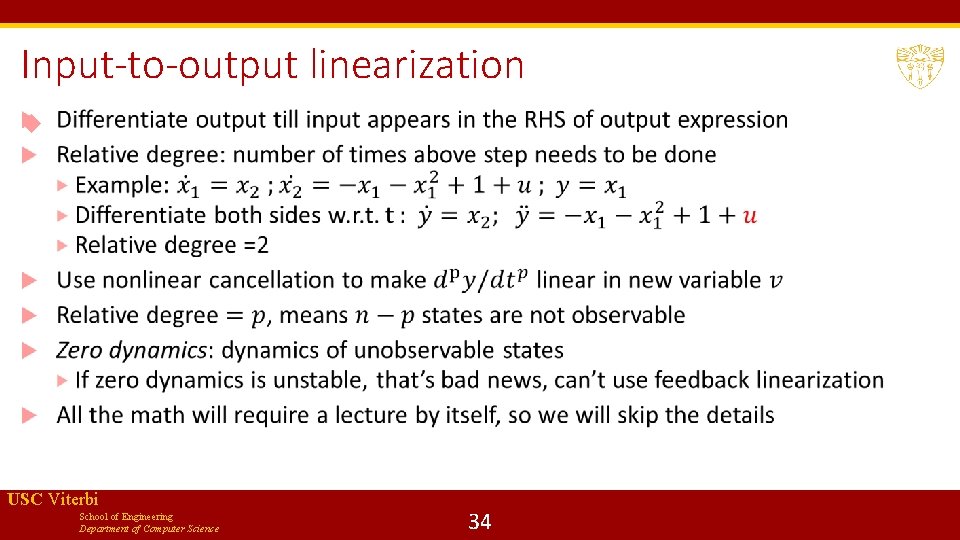
Input-to-output linearization USC Viterbi School of Engineering Department of Computer Science 34

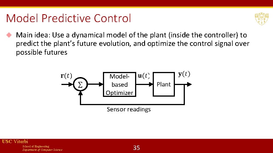
Model Predictive Control Main idea: Use a dynamical model of the plant (inside the controller) to predict the plant’s future evolution, and optimize the control signal over possible futures Modelbased Optimizer Sensor readings USC Viterbi School of Engineering Department of Computer Science 35 Plant

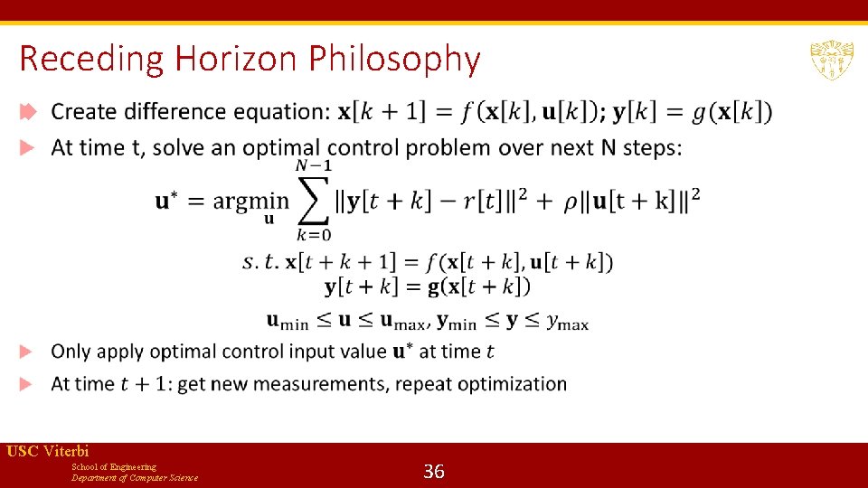
Receding Horizon Philosophy USC Viterbi School of Engineering Department of Computer Science 36

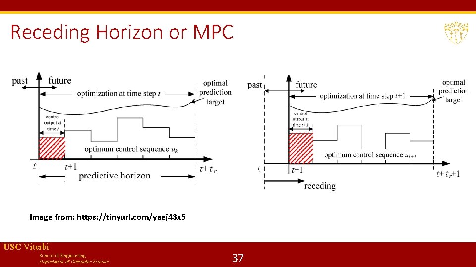
Receding Horizon or MPC Image from: https: //tinyurl. com/yaej 43 x 5 USC Viterbi School of Engineering Department of Computer Science 37

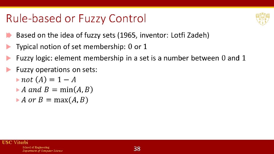
Rule-based or Fuzzy Control USC Viterbi School of Engineering Department of Computer Science 38

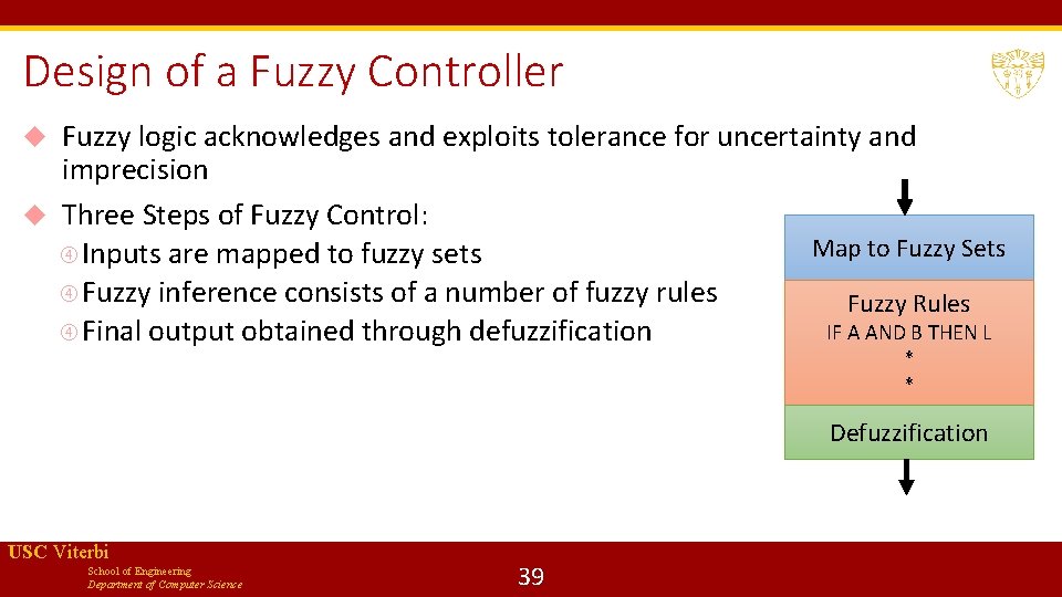
Design of a Fuzzy Controller Fuzzy logic acknowledges and exploits tolerance for uncertainty and imprecision Three Steps of Fuzzy Control: Map to Fuzzy Sets Inputs are mapped to fuzzy sets Fuzzy inference consists of a number of fuzzy rules Fuzzy Rules IF A AND B THEN L Final output obtained through defuzzification * * Defuzzification USC Viterbi School of Engineering Department of Computer Science 39

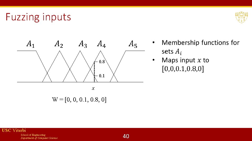
Fuzzing inputs 0. 8 0. 1 W = [0, 0, 0. 1, 0. 8, 0] USC Viterbi School of Engineering Department of Computer Science 40

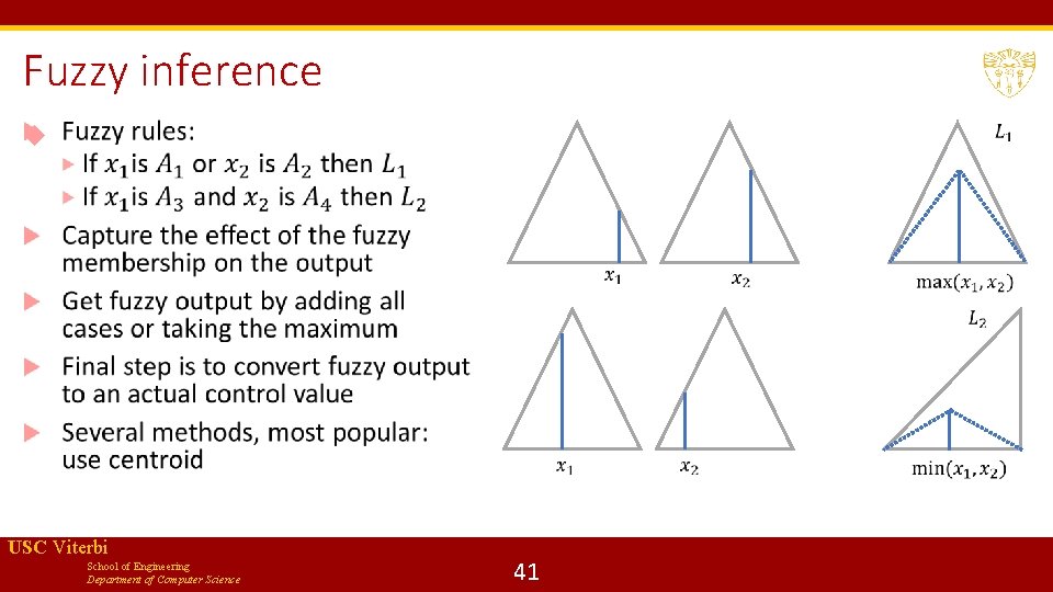
Fuzzy inference USC Viterbi School of Engineering Department of Computer Science 41

Observer design USC Viterbi School of Engineering Department of Computer Science 42

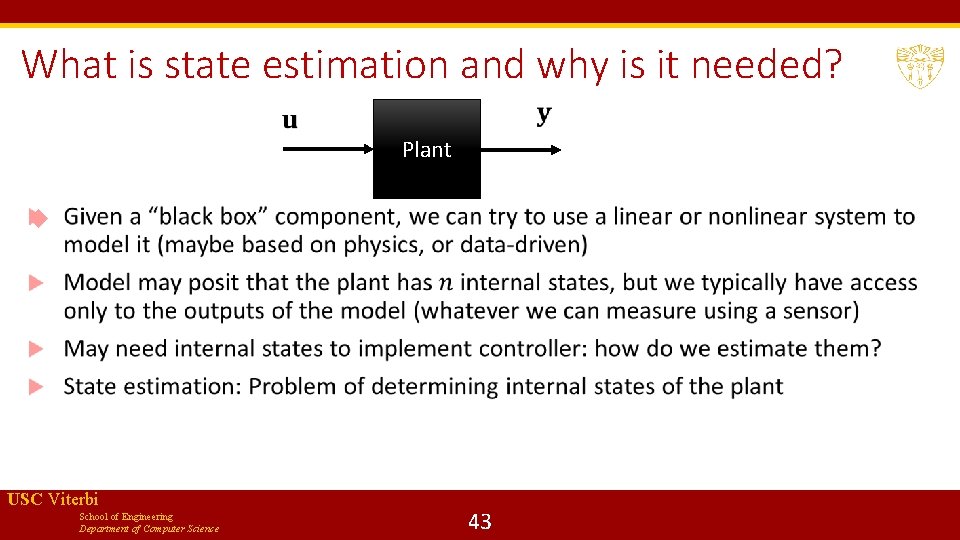
What is state estimation and why is it needed? Plant USC Viterbi School of Engineering Department of Computer Science 43

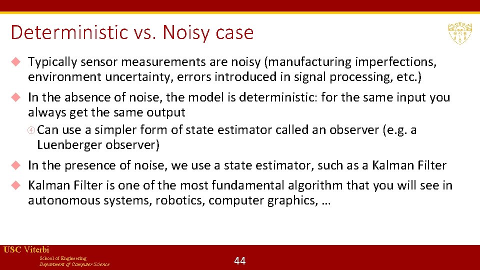
Deterministic vs. Noisy case Typically sensor measurements are noisy (manufacturing imperfections, environment uncertainty, errors introduced in signal processing, etc. ) In the absence of noise, the model is deterministic: for the same input you always get the same output Can use a simpler form of state estimator called an observer (e. g. a Luenberger observer) In the presence of noise, we use a state estimator, such as a Kalman Filter is one of the most fundamental algorithm that you will see in autonomous systems, robotics, computer graphics, … USC Viterbi School of Engineering Department of Computer Science 44

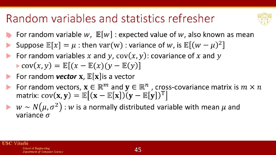
Random variables and statistics refresher USC Viterbi School of Engineering Department of Computer Science 45

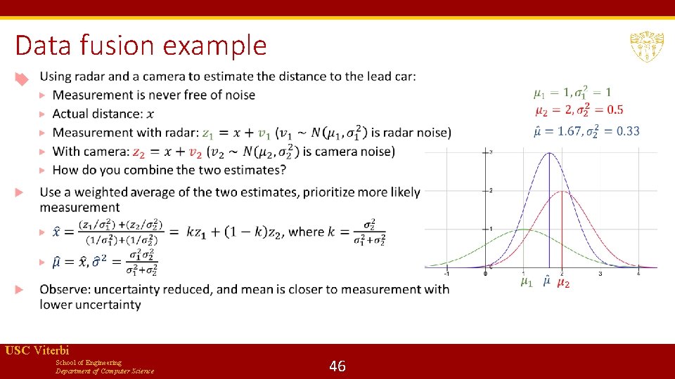
Data fusion example USC Viterbi School of Engineering Department of Computer Science 46

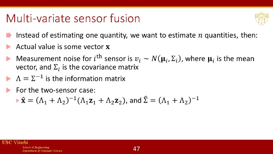
Multi-variate sensor fusion USC Viterbi School of Engineering Department of Computer Science 47

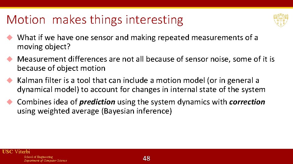
Motion makes things interesting What if we have one sensor and making repeated measurements of a moving object? Measurement differences are not all because of sensor noise, some of it is because of object motion Kalman filter is a tool that can include a motion model (or in general a dynamical model) to account for changes in internal state of the system Combines idea of prediction using the system dynamics with correction using weighted average (Bayesian inference) USC Viterbi School of Engineering Department of Computer Science 48

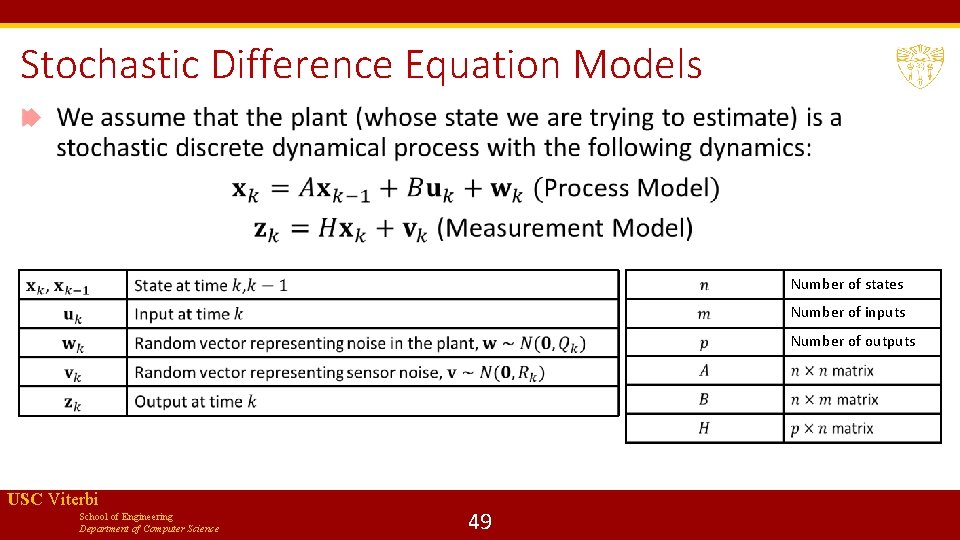
Stochastic Difference Equation Models Number of states Number of inputs Number of outputs USC Viterbi School of Engineering Department of Computer Science 49

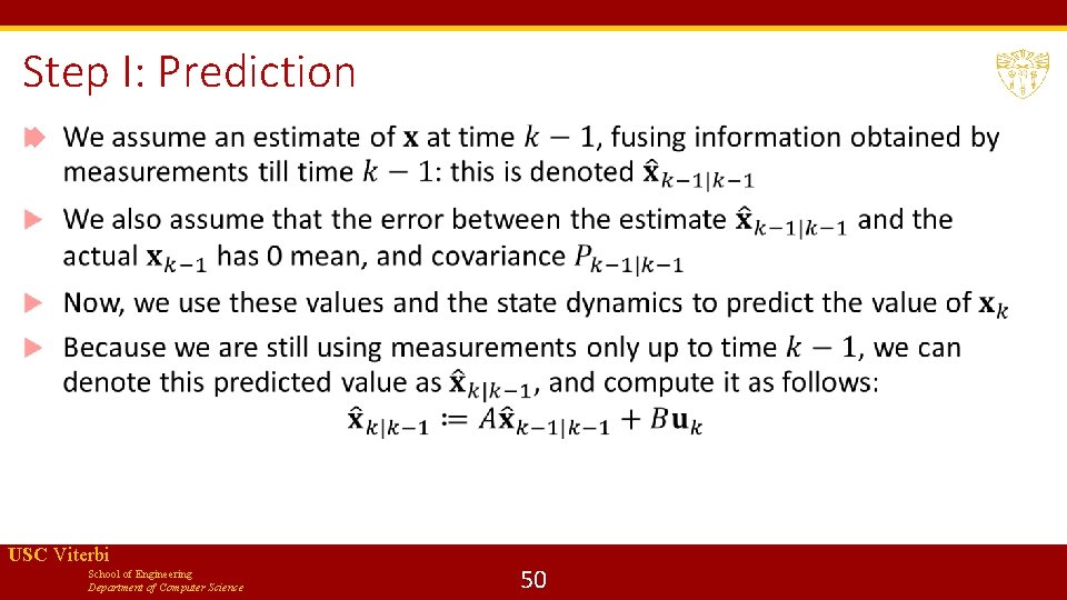
Step I: Prediction USC Viterbi School of Engineering Department of Computer Science 50

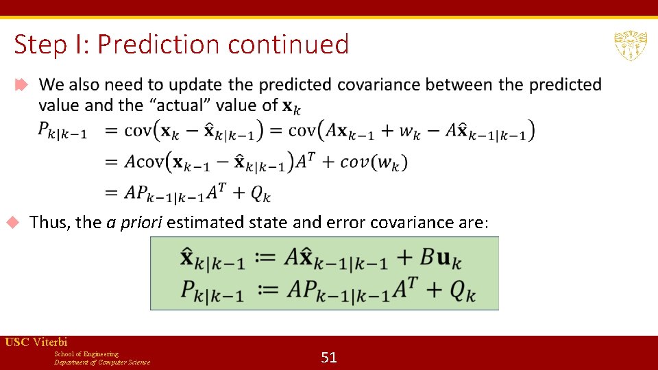
Step I: Prediction continued Thus, the a priori estimated state and error covariance are: USC Viterbi School of Engineering Department of Computer Science 51

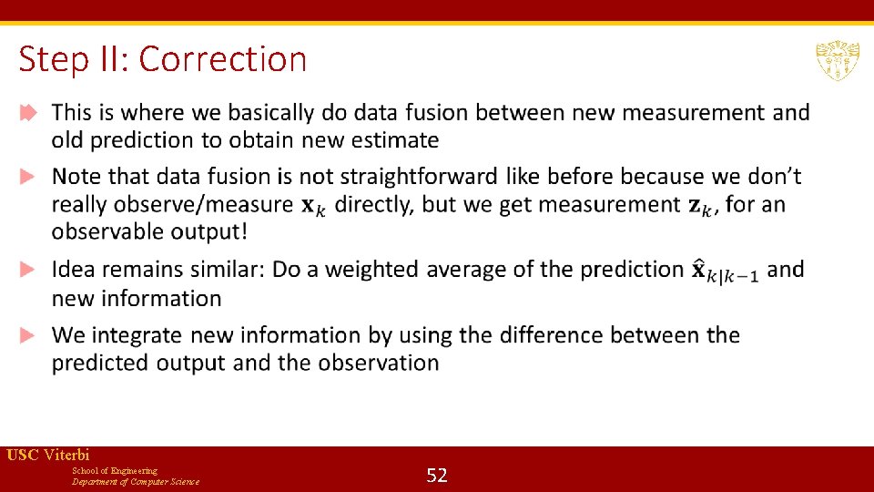
Step II: Correction USC Viterbi School of Engineering Department of Computer Science 52

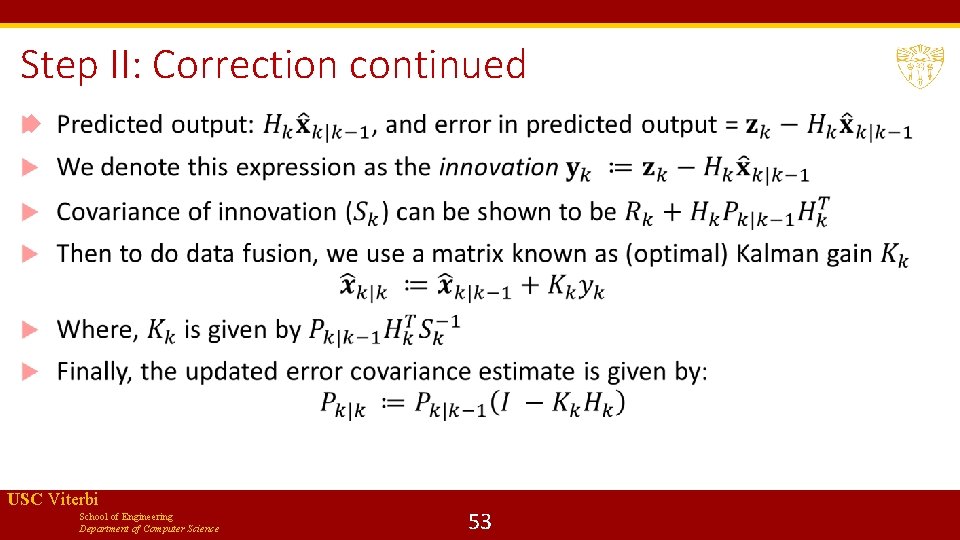
Step II: Correction continued USC Viterbi School of Engineering Department of Computer Science 53

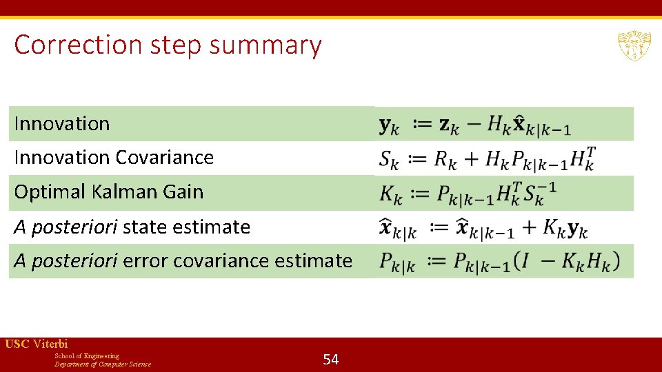
Correction step summary Innovation Covariance Optimal Kalman Gain A posteriori state estimate A posteriori error covariance estimate USC Viterbi School of Engineering Department of Computer Science 54

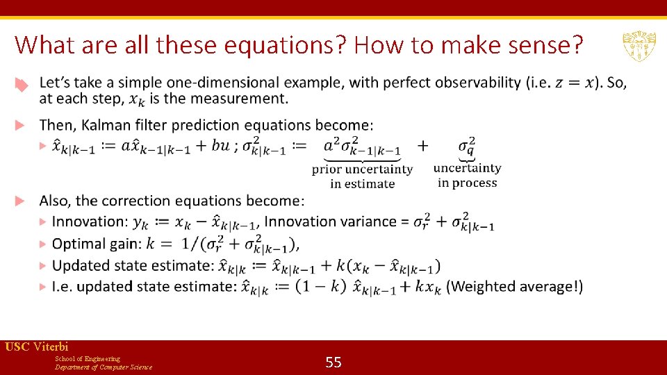
What are all these equations? How to make sense? USC Viterbi School of Engineering Department of Computer Science 55

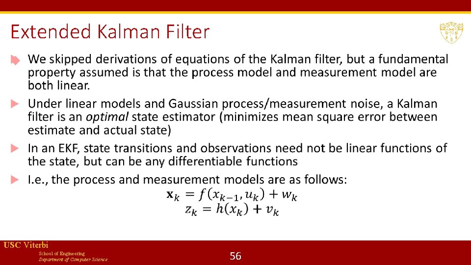
Extended Kalman Filter USC Viterbi School of Engineering Department of Computer Science 56

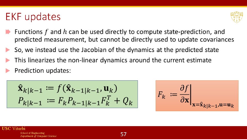
EKF updates USC Viterbi School of Engineering Department of Computer Science 57

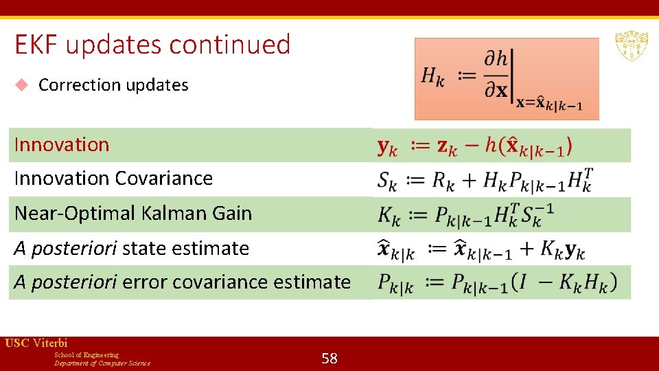
EKF updates continued Correction updates Innovation Covariance Near-Optimal Kalman Gain A posteriori state estimate A posteriori error covariance estimate USC Viterbi School of Engineering Department of Computer Science 58

EKF drawbacks EKF is not in general an optimal estimator If initial state estimate is wrong filter may diverge quickly : estimates will no longer agree with reality/observations Estimated covariance matrix tends to underestimate true covariance Yet, EKF remains widely used! GPS, most navigation systems, Openpilot (for drones), Pixhawk (mobile robots), etc. EKF in practice requires lot of “expert tuning of parameters” Most parameters occur in process models, covariance matrices, gains etc. EKF improvement: Unscented Kalman Filter USC Viterbi School of Engineering Department of Computer Science 59

End of Module 1 Models of Computation Synchronous, Asynchronous Models Timed models and Dynamical System Models Hybrid Models Basics of Linear and Nonlinear Control, Observer Design USC Viterbi School of Engineering Department of Computer Science 60

Next lecture Start with Macro-Module 2: Formal Specification and Verification USC Viterbi School of Engineering Department of Computer Science 61