Automating the Analysis of Simulation Output Data Katy

Automating the Analysis of Simulation Output Data Katy Hoad (kathryn. hoad@wbs. ac. uk), Stewart Robinson, Ruth Davies, Mark Elder Funded by EPSRC and SIMUL 8 Corporation

Project Web Site: http: //www. wbs. ac. uk/go/autosimoa INTRODUCTION Appropriate use of a simulation model requires accurate measures of model performance. This in turn, requires decisions concerning three key areas: warm-up, run-length and number of replications. These decisions require specific skills in statistics. Most Simulation software provides little or no guidance to users on making these important decisions. The Auto. Sim. OA Project is investigating the development of a methodology for automatically advising a simulation user on these three key decisions:

• How long a warm-up is required? • How long a run length is required? • How many replications should be run? PROJECT OBJECTIVES • To determine the most appropriate methods for automating simulation output analysis • To determine the effectiveness of the analysis methods • To revise the methods where necessary in order to improve their effectiveness and capacity for automation • To propose a procedure for automated output analysis of warm-up, replications and run-length (Only looking at analysis of a single scenario)

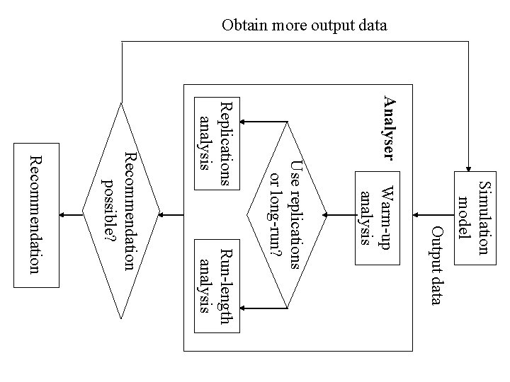
Obtain more output data Analyser Simulation model Output data Warm-up analysis Run-length analysis Use replications or long-run? Replications analysis Recommendation possible? Recommendation

Task 1: MODEL CLASSIFICATION Creating A Standard Set of Model Outputs At the beginning of this project it was decided that a standard set of model outputs was required for testing the output analysis methods. As this was not readily available in the literature it was proposed to create a representative and sufficient set of models / data output that could be used in discrete event simulation research by this project and other researchers. A set of artificial data sets were developed and a range of ‘real’ simulation models gathered together.

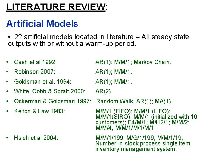
LITERATURE REVIEW: Artificial Models • 22 artificial models located in literature – All steady state outputs with or without a warm-up period. • Cash et al 1992: AR(1); M/M/1; Markov Chain. • Robinson 2007: AR(1); M/M/1. • Goldsman et al. 1994: AR(1); M/M/1. • White, Cobb & Spratt 2000: AR(2). • Ockerman & Goldsman 1997: Random Walk; AR(1); MA(1). • Kelton & Law 1983: M/M/1 (FIFO); M/M/1 (LIFO); M/M/1(SIRO); M/M/1 (initialized with 10 customers); E 4/M/1; M/H 2/1; M/M/2; M/M/4; M/M/1/M/1. • Hsieh et al 2004: M/M/1/199; M/G/1/199; M/M/1/19; Number-in-stock process single item inventory management system.

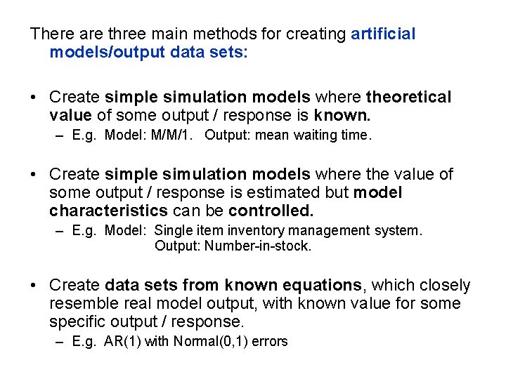
There are three main methods for creating artificial models/output data sets: • Create simple simulation models where theoretical value of some output / response is known. – E. g. Model: M/M/1. Output: mean waiting time. • Create simple simulation models where the value of some output / response is estimated but model characteristics can be controlled. – E. g. Model: Single item inventory management system. Output: Number-in-stock. • Create data sets from known equations, which closely resemble real model output, with known value for some specific output / response. – E. g. AR(1) with Normal(0, 1) errors

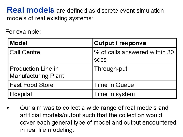
Real models are defined as discrete event simulation models of real existing systems: For example: • Model Call Centre Output / response % of calls answered within 30 secs Production Line in Manufacturing Plant Fast Food Store Hospital Through-put Time in Queue Time in system Our aim was to collect a wide range of real models and artificial models/output such that the collection would cover each general type of model and output encountered in real life modeling.

METHODOLOGY: It was determined that model output fell into two main categories or groups: Ø Transient (including out-of-control trend) Ø Steady-state (including steady-state cycle) 9 other characteristics of models and output data sets were chosen to be used to categorize the models/output within these two main groups:

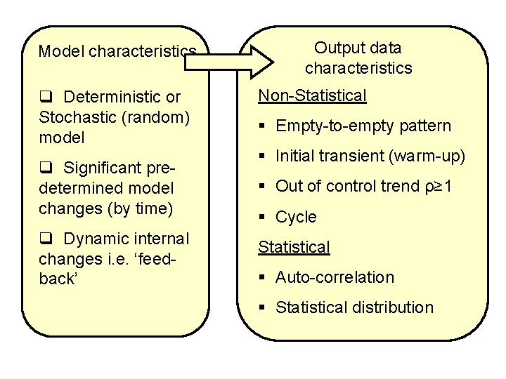
Model characteristics q Deterministic or Stochastic (random) model q Significant predetermined model changes (by time) q Dynamic internal changes i. e. ‘feedback’ Output data characteristics Non-Statistical § Empty-to-empty pattern § Initial transient (warm-up) § Out of control trend ρ≥ 1 § Cycle Statistical § Auto-correlation § Statistical distribution

After collection or creation of model / output the data output sets were identified as one of 5 types: Steady state; Steady state cycle; Transient; Out-of-Control Each type was statistically analysed as follows: 1. Steady State: Subtract mean from output data. Test residuals for Auto-correlation and Normality. 2. Steady State Cycle: Run model for many cycles. Take mean of each cycle to create a new time series. Subtract mean from this new output data. Test residuals for Auto-correlation and Normality. 3. Transient: Test for Auto-correlation on output data. Run many replications (1000) Take mean of each replication to create new (non auto-correlated) data series. Test for what type of statistical distribution best fits this new data series. 4. Out-Of-Control: Plot data

RESULTS: • The following distributions were found to be a ‘good’ fit to the various transient data output. Normal, Beta, Pearson 5, Log. Normal, Weibull, Gamma, Pearson 6, Erlang, Chi squared No fits could be found for two of the transient data sets. • Classification tables were drawn up

DISCUSSION: YOUR COMMENTS APPRECIATED Ø Using our chosen classification criteria, we have classified a complete set of possible models / output: But are these criteria sufficient? Ø Main model/output types missing from our collection: • Transient with warm-up. • Deterministic transient. • Cycle with warm-up Are these missing model criteria feasible?

Ø Justification of selection of model results / output e. g. through-put etc… Picked most likely output result for each model, using already programmed results collection when feasible. Ø Future intentions: To create artificial data sets for each category that is missing a real model example. To test chosen (automatic) simulation output analysis methods on each category of model / output.

Task 2: NUMBER OF REPLICATIONS

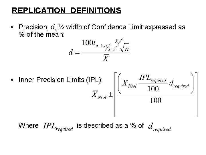
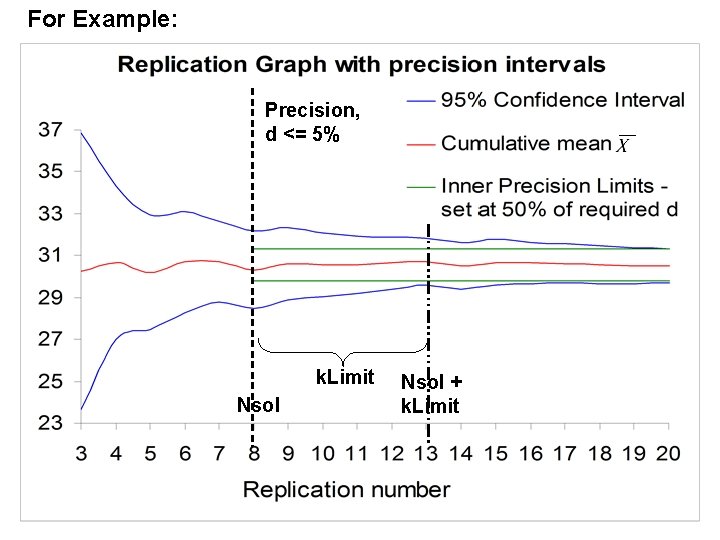
REPLICATION DEFINITIONS • Precision, d, ½ width of Confidence Limit expressed as % of the mean: • Inner Precision Limits (IPL): Where is described as a % of

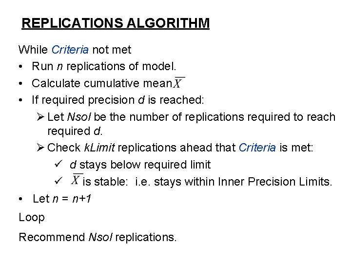
REPLICATIONS ALGORITHM While Criteria not met • Run n replications of model. • Calculate cumulative mean • If required precision d is reached: Ø Let Nsol be the number of replications required to reach required d. Ø Check k. Limit replications ahead that Criteria is met: ü d stays below required limit ü is stable: i. e. stays within Inner Precision Limits. • Let n = n+1 Loop Recommend Nsol replications.

For Example: Precision, d <= 5% k. Limit Nsol + k. Limit

FUTURE WORK • To determine the most appropriate methods for automating warm-up and run-length analysis • To determine the effectiveness of the analysis methods • To revise the methods where necessary in order to improve their effectiveness and capacity for automation • To propose a procedure for automated output analysis of warm-up and run-length