Automatic Speech Recognition ILVB2006 Tutorial 1 The Noisy

Automatic Speech Recognition ILVB-2006 Tutorial 1

The Noisy Channel Model • Automatic speech recognition (ASR) is a process by which an acoustic speech signal is converted into a set of words [Rabiner et al. , 1993] • The noisy channel model [Lee et al. , 1996] – Acoustic input considered a noisy version of a source sentence Noisy Channel Source sentence Noisy sentence 버스 정류장이 어디에 있나요? ILVB-2006 Tutorial Decoder Guess at original sentence 버스 정류장이 어디에 있나요? 2

The Noisy Channel Model • What is the most likely sentence out of all sentences in the language L given some acoustic input O? • Treat acoustic input O as sequence of individual observations – O = o 1, o 2, o 3, …, ot • Define a sentence as a sequence of words: – W = w 1, w 2, w 3, …, wn Bayes rule Golden rule ILVB-2006 Tutorial 3

Speech Recognition Architecture Meets Noisy Channel 버스 정류장이 어디에 있나요? Speech Signals 버스 정류장이 어디에 있나요? Feature Extraction Decoding Word Sequence Network Construction Speech DB HMM Estimation G 2 P Text Corpora ILVB-2006 Tutorial LM Estimation 4 Acoustic Pronunciation Model Language Model

Feature Extraction • The Mel-Frequency Cepstrum Coefficients (MFCC) is a popular choice [Paliwal, 1992] Preemphasis/ Hamming Window X(n) FFT (Fast Fourier Transform) Mel-scale filter bank log|. | DCT (Discrete Cosine Transform) – Frame size : 25 ms / Frame rate : 10 ms 25 ms. . . 10 ms a 1 a 2 a 3 – 39 feature per 10 ms frame – Absolute : Log Frame Energy (1) and MFCCs (12) – Delta : First-order derivatives of the 13 absolute coefficients – Delta-Delta : Second-order derivatives of the 13 absolute coefficients ILVB-2006 Tutorial 5 MFCC (12 -Dimension)

Acoustic Model • Provide P(O|Q) = P(features|phone) • Modeling Units [Bahl et al. , 1986] – Context-independent : Phoneme – Context-dependent : Diphone, Triphone, Quinphone – p. L-p+p. R : left-right context triphone • Typical acoustic model [Juang et al. , 1986] – Continuous-density Hidden Markov Model – Distribution : Gaussian Mixture – HMM Topology : 3 -state left-to-right model for each phone, 1 -state for silence or pause bj(x) codebook ILVB-2006 Tutorial 6

Pronunciation Model • Provide P(Q|W) = P(phone|word) • Word Lexicon [Hazen et al. , 2002] – Map legal phone sequences into words according to phonotactic rules – G 2 P (Grapheme to phoneme) : Generate a word lexicon automatically – Several word may have multiple pronunciations • Example – Tomato 0. 2 [ow] 0. 5 1. 0 [ey] 1. 0 [m] [t] 0. 8 [ah] 1. 0 [t] 0. 5 [aa] 1. 0 – P([towmeytow]|tomato) = P([towmaatow]|tomato) = 0. 1 – P([tahmeytow]|tomato) = P([tahmaatow]|tomato) = 0. 4 ILVB-2006 Tutorial 7 [ow]

Training • Training process [Lee et al. , 1996] Speech DB Feature Extraction Baum-Welch Re-estimation yes Converged? no HMM • Network for training Sentence HMM Word HMM ONE Phone HMM W ILVB-2006 Tutorial ONE TWO THREE ONE 8 W 1 TWO AH 2 3 THREE ONE N End

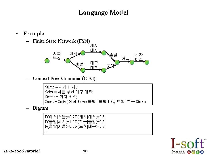
Language Model • Provide P(W) ; the probability of the sentence [Beaujard et al. , 1999] – We saw this was also used in the decoding process as the probability of transitioning from one word to another. – Word sequence : W = w 1, w 2, w 3, …, wn – The problem is that we cannot reliably estimate the conditional word probabilities, for all words and all sequence lengths in a given language – n-gram Language Model – n-gram language models use the previous n-1 words to represent the history – Bi-grams are easily incorporated in a viterbi search ILVB-2006 Tutorial 9

Network Construction • Expanding every word to state level, we get a search network [Demuynck et al. , 1997] Acoustic Model Pronunciation Model I 일 I L 이 I 삼 S 사 S S A M L 이 A LM is applied 일 M 사 A 삼 Intra-word transition start Language Model 이 Search Network Word transition end I P(이|x) P(일 |x) I L P(사|x) Between-word transition S A 일 사 P(삼|x) S ILVB-2006 Tutorial 11 A M 삼

Decoding • Find • Viterbi Search : Dynamic Programming – Token Passing Algorithm [Young et al. , 1989] • • ILVB-2006 Tutorial Initialize all states with a token with a null history and the likelihood that it’s a start state For each frame ak – For each token t in state s with probability P(t), history H – For each state r – Add new token to s with probability P(t) Ps, r Pr(ak), and history s. H 12

Decoding • Pruning [Young et al. , 1996] – Entire search space for Viterbi search is much too large – Solution is to prune tokens for paths whose score is too low – Typical method is to use: – histogram: only keep at most n total hypotheses – beam: only keep hypotheses whose score is a fraction of best score • N-best Hypotheses and Word Graphs – Keep multiple tokens and return n-best paths/scores – Can produce a packed word graph (lattice) • Multiple Pass Decoding – Perform multiple passes, applying successively more fine-grained language models ILVB-2006 Tutorial 13

Large Vocabulary Continuous Speech Recognition (LVCSR) • Decoding continuous speech over large vocabulary – Computationally complex because of huge potential search space • Weighted Finite State Transducers (WFST) [Mohri et al. , 2002] – Efficiency in time and space Word : Sentence WFST Phone : Word WFST HMM : Phone WFST State : HMM WFST • Dynamic Decoding – On-demand network constructions – Much less memory requirements ILVB-2006 Tutorial 14 Combination Optimization Search Network