Automatic Selection of Loop Scheduling Algorithms Using Reinforcement
![Automatic Selection of Loop Scheduling Algorithms Using Reinforcement Learning Mahbubur Rashid[1, 2], Ioana Banicescu[1, Automatic Selection of Loop Scheduling Algorithms Using Reinforcement Learning Mahbubur Rashid[1, 2], Ioana Banicescu[1,](https://slidetodoc.com/presentation_image/fb2c80cfb54c040a7c31a763d206f413/image-1.jpg)







- Slides: 46
![Automatic Selection of Loop Scheduling Algorithms Using Reinforcement Learning Mahbubur Rashid1 2 Ioana Banicescu1 Automatic Selection of Loop Scheduling Algorithms Using Reinforcement Learning Mahbubur Rashid[1, 2], Ioana Banicescu[1,](https://slidetodoc.com/presentation_image/fb2c80cfb54c040a7c31a763d206f413/image-1.jpg)
Automatic Selection of Loop Scheduling Algorithms Using Reinforcement Learning Mahbubur Rashid[1, 2], Ioana Banicescu[1, 2], Ricolindo L. Cariño[3] [1]Department of Computer Science and Engineering [2]Center for Computational Sciences – HPC 2 [3]Center for Advanced Vehicular Systems – HPC 2 Mississippi State University Partial support from the NSF Grants: 9984465, 0085969, 0081303, 0132618, and 0082979.

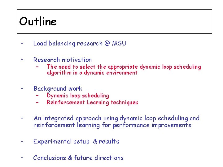
Outline • Load balancing research @ MSU • Research motivation • Background work • An integrated approach using dynamic loop scheduling and reinforcement learning for performance improvements • Experimental setup & results • Conclusions & future directions – – – The need to select the appropriate dynamic loop scheduling algorithm in a dynamic environment Dynamic loop scheduling Reinforcement Learning techniques

Load Balancing Research @ MSU

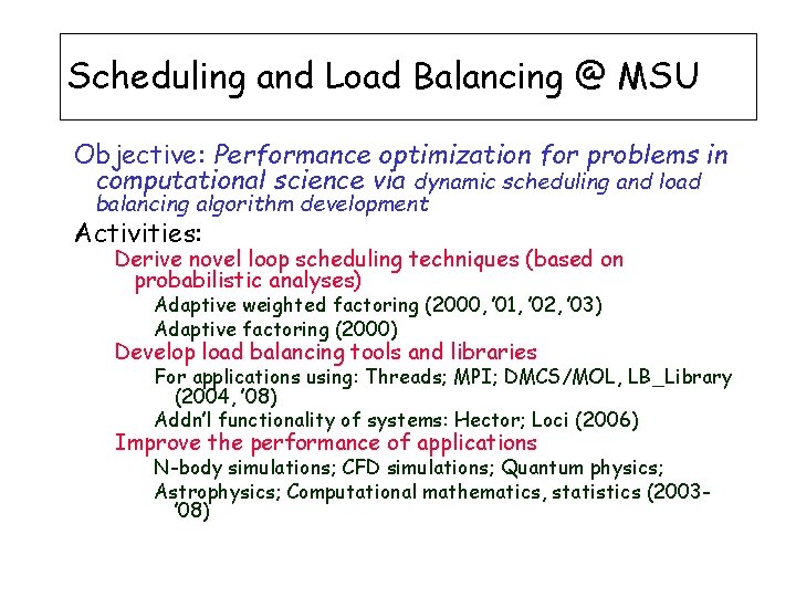
Scheduling and Load Balancing @ MSU Objective: Performance optimization for problems in computational science via dynamic scheduling and load balancing algorithm development Activities: Derive novel loop scheduling techniques (based on probabilistic analyses) Adaptive weighted factoring (2000, ’ 01, ’ 02, ’ 03) Adaptive factoring (2000) Develop load balancing tools and libraries For applications using: Threads; MPI; DMCS/MOL, LB_Library (2004, ’ 08) Addn’l functionality of systems: Hector; Loci (2006) Improve the performance of applications N-body simulations; CFD simulations; Quantum physics; Astrophysics; Computational mathematics, statistics (2003’ 08)

Research Motivation

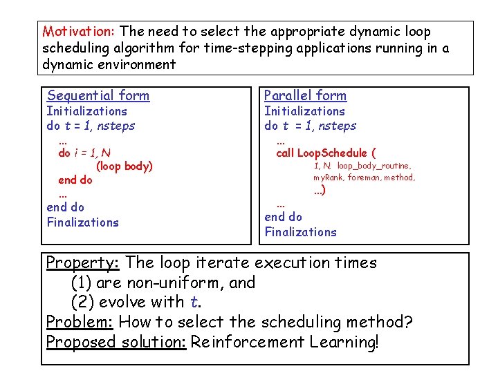
Motivation: The need to select the appropriate dynamic loop scheduling algorithm for time-stepping applications running in a dynamic environment Sequential form Initializations do t = 1, nsteps … do i = 1, N (loop body) end do … end do Finalizations Parallel form Initializations do t = 1, nsteps … call Loop. Schedule ( 1, N, loop_body_routine, my. Rank, foreman, method, … …) end do Finalizations Property: The loop iterate execution times (1) are non-uniform, and (2) evolve with t. Problem: How to select the scheduling method? Proposed solution: Reinforcement Learning!

Background Work

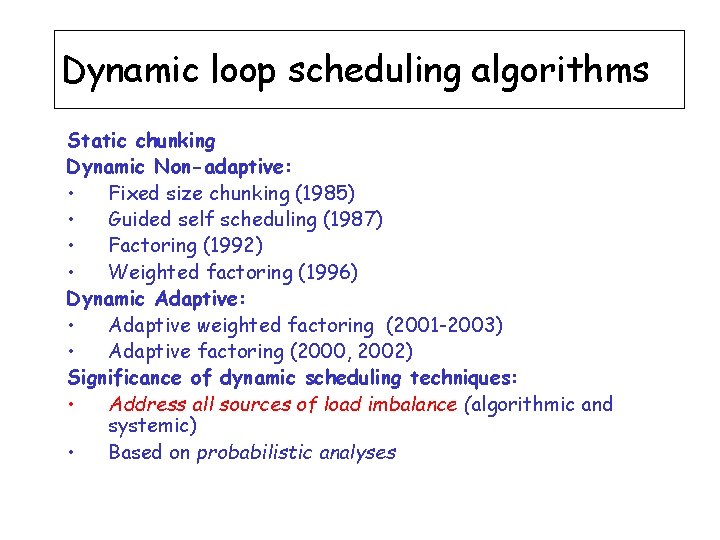
Dynamic loop scheduling algorithms Static chunking Dynamic Non-adaptive: • Fixed size chunking (1985) • Guided self scheduling (1987) • Factoring (1992) • Weighted factoring (1996) Dynamic Adaptive: • Adaptive weighted factoring (2001 -2003) • Adaptive factoring (2000, 2002) Significance of dynamic scheduling techniques: • Address all sources of load imbalance (algorithmic and systemic) • Based on probabilistic analyses

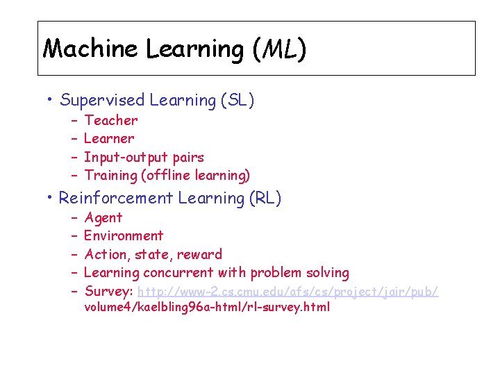
Machine Learning (ML) • Supervised Learning (SL) – – Teacher Learner Input-output pairs Training (offline learning) • Reinforcement Learning (RL) – – – Agent Environment Action, state, reward Learning concurrent with problem solving Survey: http: //www-2. cs. cmu. edu/afs/cs/project/jair/pub/ volume 4/kaelbling 96 a-html/rl-survey. html

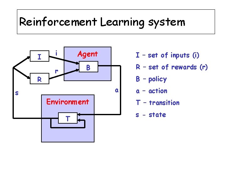
Reinforcement Learning system I R s i Agent I – set of inputs (i) R – set of rewards (r) B r B – policy a Environment T a – action T – transition s - state

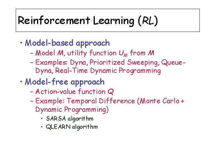
Reinforcement Learning (RL) • Model-based approach – Model M, utility function UM from M – Examples: Dyna, Prioritized Sweeping, Queue. Dyna, Real-Time Dynamic Programming • Model-free approach – Action-value function Q – Example: Temporal Difference (Monte Carlo + Dynamic Programming) • SARSA algorithm • QLEARN algorithm

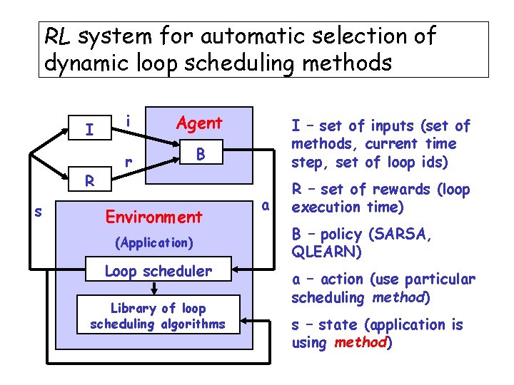
RL system for automatic selection of dynamic loop scheduling methods I R s i Agent r I – set of inputs (set of methods, current time step, set of loop ids) B Environment (Application) Loop scheduler Library of loop scheduling algorithms a R – set of rewards (loop execution time) B – policy (SARSA, QLEARN) a – action (use particular scheduling method) s – state (application is using method)

Research Approach

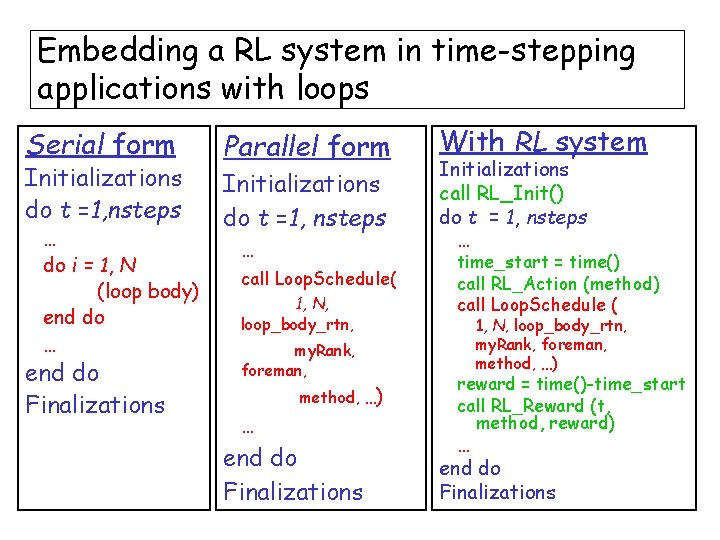
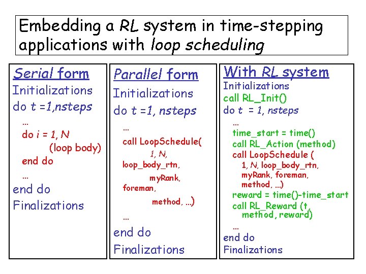
Embedding a RL system in time-stepping applications with loops Serial form Initializations do t =1, nsteps … do i = 1, N (loop body) end do … end do Finalizations Parallel form Initializations do t =1, nsteps … call Loop. Schedule( 1, N, loop_body_rtn, my. Rank, foreman, method, …) … end do Finalizations With RL system Initializations call RL_Init() do t = 1, nsteps … time_start = time() call RL_Action (method) call Loop. Schedule ( 1, N, loop_body_rtn, my. Rank, foreman, method, …) reward = time()-time_start call RL_Reward (t, method, reward) … end do Finalizations

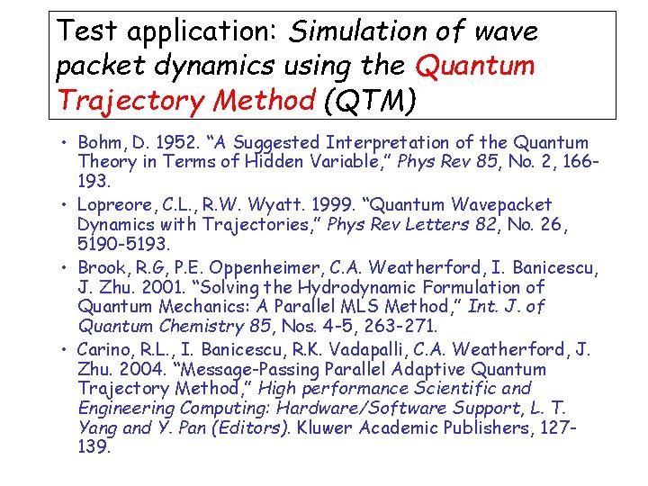
Test application: Simulation of wave packet dynamics using the Quantum Trajectory Method (QTM) • Bohm, D. 1952. “A Suggested Interpretation of the Quantum Theory in Terms of Hidden Variable, ” Phys Rev 85, No. 2, 166193. • Lopreore, C. L. , R. W. Wyatt. 1999. “Quantum Wavepacket Dynamics with Trajectories, ” Phys Rev Letters 82, No. 26, 5190 -5193. • Brook, R. G, P. E. Oppenheimer, C. A. Weatherford, I. Banicescu, J. Zhu. 2001. “Solving the Hydrodynamic Formulation of Quantum Mechanics: A Parallel MLS Method, ” Int. J. of Quantum Chemistry 85, Nos. 4 -5, 263 -271. • Carino, R. L. , I. Banicescu, R. K. Vadapalli, C. A. Weatherford, J. Zhu. 2004. “Message-Passing Parallel Adaptive Quantum Trajectory Method, ” High performance Scientific and Engineering Computing: Hardware/Software Support, L. T. Yang and Y. Pan (Editors). Kluwer Academic Publishers, 127139.

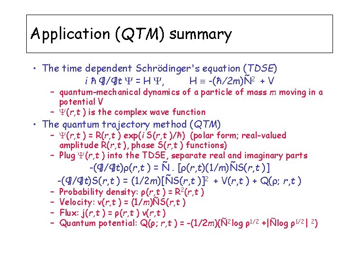
Application (QTM) summary • The time dependent Schrödinger's equation (TDSE) i ħ ¶/¶t = H , H -(ħ/2 m)Ñ 2 + V – quantum-mechanical dynamics of a particle of mass m moving in a potential V – (r, t ) is the complex wave function • The quantum trajectory method (QTM) – (r, t ) = R(r, t ) exp(i S(r, t )/ħ) (polar form; real-valued amplitude R(r, t ), phase S(r, t ) functions) – Plug (r, t ) into the TDSE, separate real and imaginary parts – – -(¶/¶t)ρ(r, t ) = Ñ. [ρ(r, t)(1/m)ÑS(r, t )] -(¶/¶t)S(r, t ) = (1/2 m)[ÑS(r, t )]2 + V(r, t ) + Q(ρ; r, t ) Probability density: ρ(r, t ) = R 2(r, t ) Velocity: v(r, t ) = (1/m)ÑS(r, t ) Flux: j(r, t ) = ρ(r, t ) v(r, t ) Quantum potential: Q(ρ; r, t ) = -(1/2 m)(Ñ 2 log ρ1/2 +|Ñlog ρ1/2| 2)

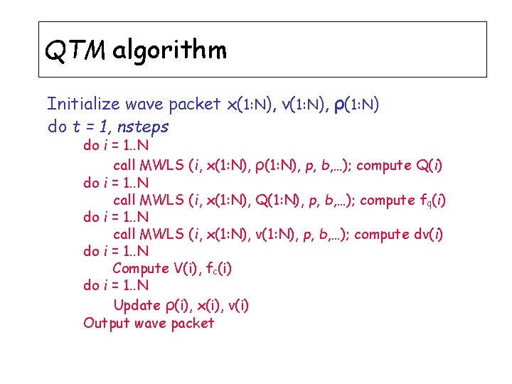
QTM algorithm Initialize wave packet x(1: N), v(1: N), ρ(1: N) do t = 1, nsteps do i = 1. . N call MWLS (i, x(1: N), ρ(1: N), p, b, …); compute Q(i) do i = 1. . N call MWLS (i, x(1: N), Q(1: N), p, b, …); compute fq(i) do i = 1. . N call MWLS (i, x(1: N), v(1: N), p, b, …); compute dv(i) do i = 1. . N Compute V(i), fc(i) do i = 1. . N Update ρ(i), x(i), v(i) Output wave packet

Embedding a RL system in time-stepping applications with loop scheduling Serial form Initializations do t =1, nsteps … do i = 1, N (loop body) end do … end do Finalizations Parallel form Initializations do t =1, nsteps … call Loop. Schedule( 1, N, loop_body_rtn, my. Rank, foreman, method, …) … end do Finalizations With RL system Initializations call RL_Init() do t = 1, nsteps … time_start = time() call RL_Action (method) call Loop. Schedule ( 1, N, loop_body_rtn, my. Rank, foreman, method, …) reward = time()-time_start call RL_Reward (t, method, reward) … end do Finalizations

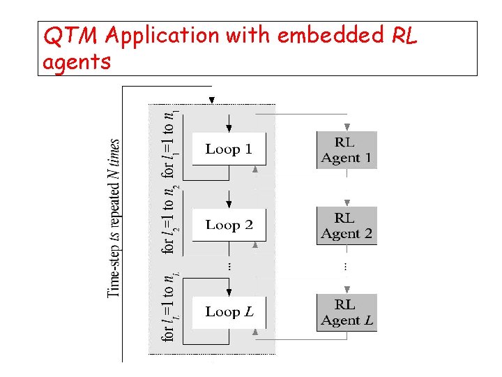
QTM Application with embedded RL agents

Experimental Setups & Results

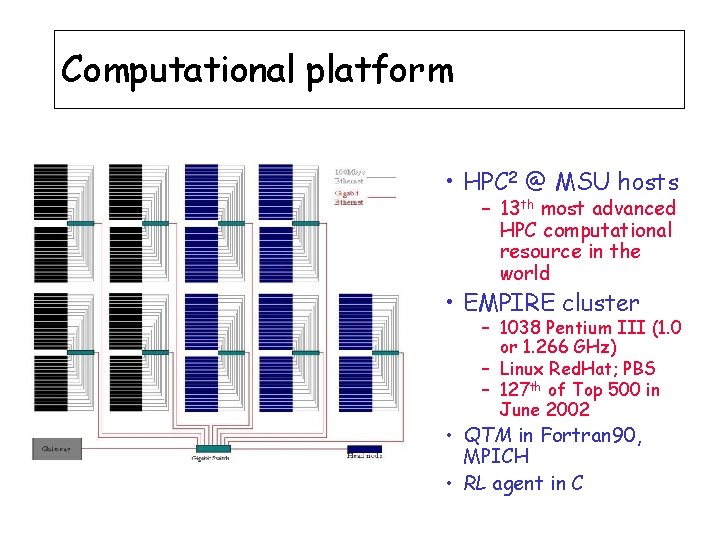
Computational platform • HPC 2 @ MSU hosts – 13 th most advanced HPC computational resource in the world • EMPIRE cluster – 1038 Pentium III (1. 0 or 1. 266 GHz) – Linux Red. Hat; PBS – 127 th of Top 500 in June 2002 • QTM in Fortran 90, MPICH • RL agent in C

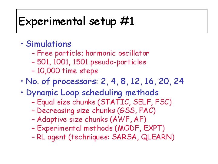
Experimental setup #1 • Simulations – Free particle; harmonic oscillator – 501, 1001, 1501 pseudo-particles – 10, 000 time steps • No. of processors: 2, 4, 8, 12, 16, 20, 24 • Dynamic Loop scheduling methods – Equal size chunks (STATIC, SELF, FSC) – Decreasing size chunks (GSS, FAC) – Adaptive size chunks (AWF, AF) – Experimental methods (MODF, EXPT) – RL agent (techniques: SARSA, QLEARN)

Experimental setup #1 (cont. ) • Hypothesis – The simulation performs better using dynamic scheduling methods with RL than dynamic scheduling methods without RL • Design – Two-factorial experiment (factors: methods, no. of processors) – Five (5) replicates – Average parallel execution time TP – Comparison via t statistic at 0. 05 significance level, using Least Squares Means

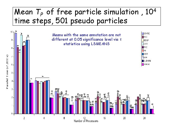
Mean TP of free particle simulation , 104 time steps, 501 pseudo particles Means with the same annotation are not different at 0. 05 significance level via t statistics using LSMEANS

Experimental setup #2 • Simulations – Free particle; harmonic oscillator – 1001 pseudo-particles – 500 time steps • No. of processors: 4, 8, 12 • Dynamic Loop scheduling methods – Equal size chunks (STATIC, SELF, FSC) – Decreasing size chunks (GSS, FAC) – Adaptive size chunks (AWF, AF) – Experimental methods (MODF, EXPT) – RL agent (techniques: SARSA, QLEARN)

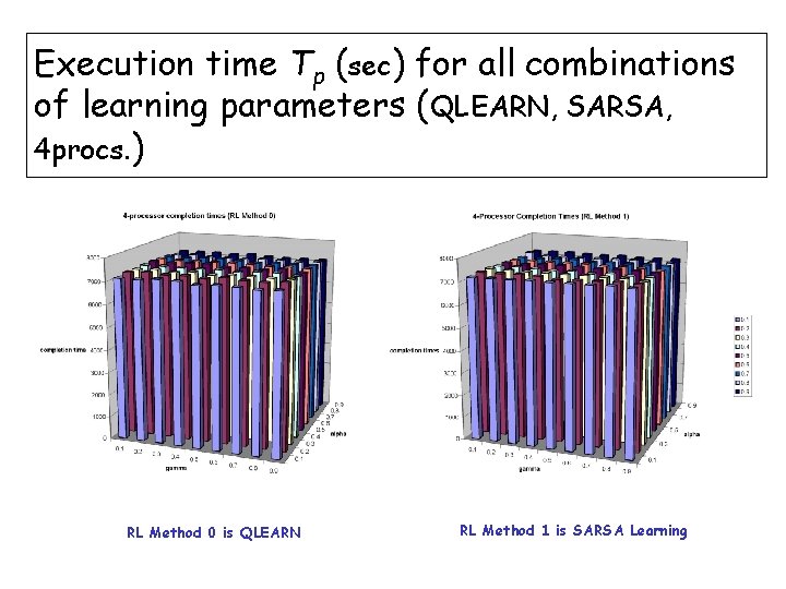
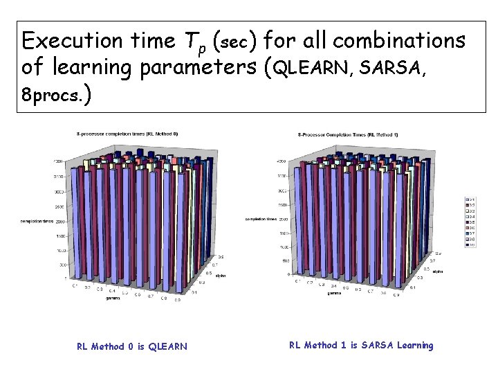
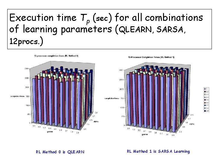
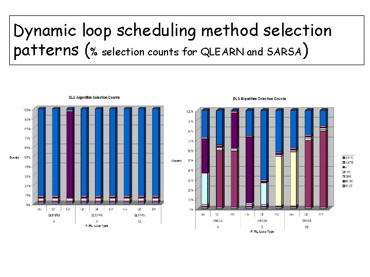
Experimental setup #2 (cont. ) • Hypothesis – The simulation performance is not sensitive to the learning parameters or the type of learning technique used in the RL agent – Each learning technique selects the dynamic loop scheduling methods in a unique pattern • Design – Two-factorial experiment (factors: methods, no. of processors) – Five (5) replicates – Average parallel execution time TP – Comparison via t statistic at 0. 05 significance level, using Least Squares Means

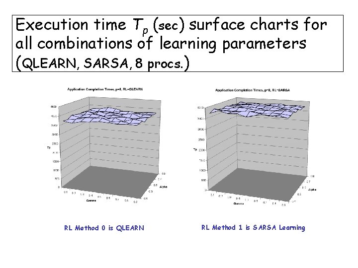
Execution time Tp (sec) for all combinations of learning parameters (QLEARN, SARSA, 4 procs. ) RL Method 0 is QLEARN RL Method 1 is SARSA Learning

Execution time Tp (sec) for all combinations of learning parameters (QLEARN, SARSA, 8 procs. ) RL Method 0 is QLEARN RL Method 1 is SARSA Learning

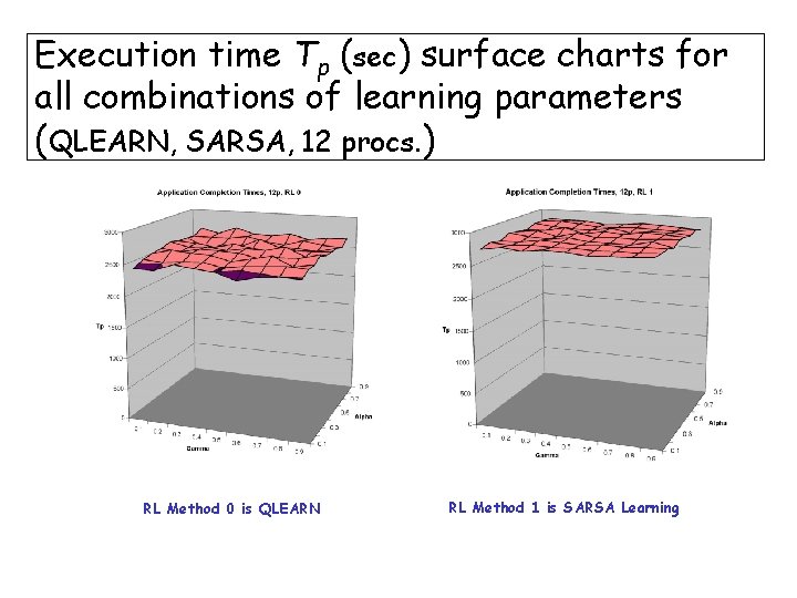
Execution time Tp (sec) for all combinations of learning parameters (QLEARN, SARSA, 12 procs. ) RL Method 0 is QLEARN RL Method 1 is SARSA Learning

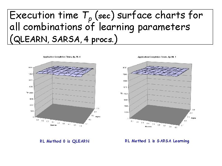
Execution time Tp (sec) surface charts for all combinations of learning parameters (QLEARN, SARSA, 4 procs. ) RL Method 0 is QLEARN RL Method 1 is SARSA Learning

Execution time Tp (sec) surface charts for all combinations of learning parameters (QLEARN, SARSA, 8 procs. ) RL Method 0 is QLEARN RL Method 1 is SARSA Learning

Execution time Tp (sec) surface charts for all combinations of learning parameters (QLEARN, SARSA, 12 procs. ) RL Method 0 is QLEARN RL Method 1 is SARSA Learning

Dynamic loop scheduling method selection patterns (% selection counts for QLEARN and SARSA)

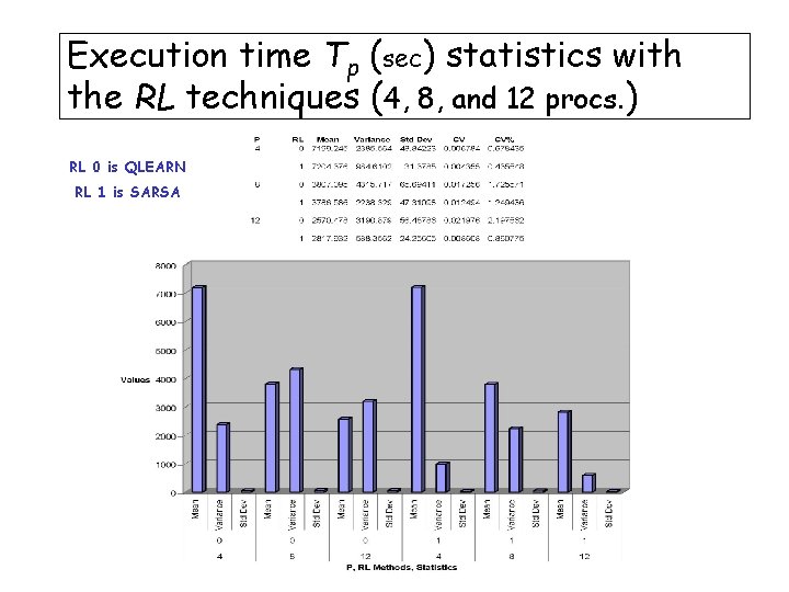
Execution time Tp (sec) statistics with the RL techniques (4, 8, and 12 procs. ) RL 0 is QLEARN RL 1 is SARSA

Conclusions & Future Directions

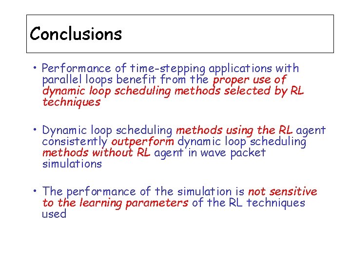
Conclusions • Performance of time-stepping applications with parallel loops benefit from the proper use of dynamic loop scheduling methods selected by RL techniques • Dynamic loop scheduling methods using the RL agent consistently outperform dynamic loop scheduling methods without RL agent in wave packet simulations • The performance of the simulation is not sensitive to the learning parameters of the RL techniques used

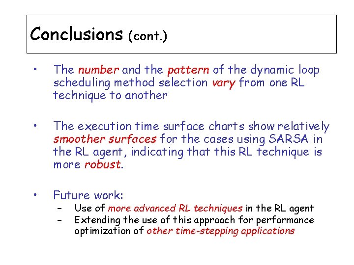
Conclusions (cont. ) • The number and the pattern of the dynamic loop scheduling method selection vary from one RL technique to another • The execution time surface charts show relatively smoother surfaces for the cases using SARSA in the RL agent, indicating that this RL technique is more robust. • Future work: – – Use of more advanced RL techniques in the RL agent Extending the use of this approach for performance optimization of other time-stepping applications

Appendix

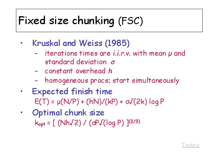
Fixed size chunking (FSC) • Kruskal and Weiss (1985) • Expected finish time • Optimal chunk size – iterations times are i. i. r. v. with mean μ and standard deviation σ – constant overhead h – homogeneous procs; start simultaneously E(T) = μ(N/P) + (h. N)/(k. P) + σ√(2 k) log P kopt = [ (Nh√ 2) / (σP√(log P) ](2/3) Index

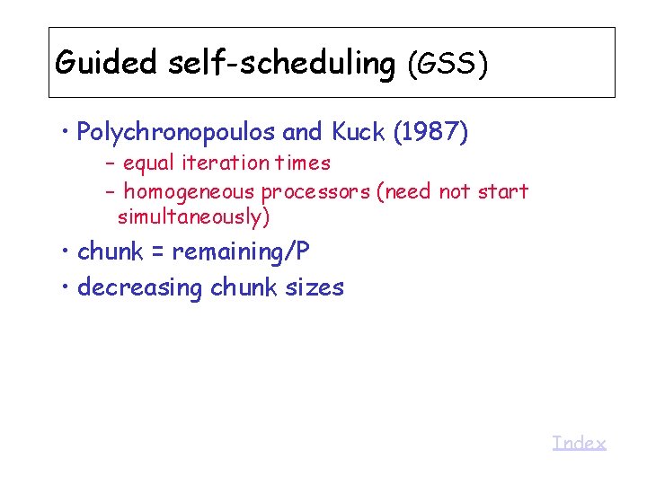
Guided self-scheduling (GSS) • Polychronopoulos and Kuck (1987) – equal iteration times – homogeneous processors (need not start simultaneously) • chunk = remaining/P • decreasing chunk sizes Index

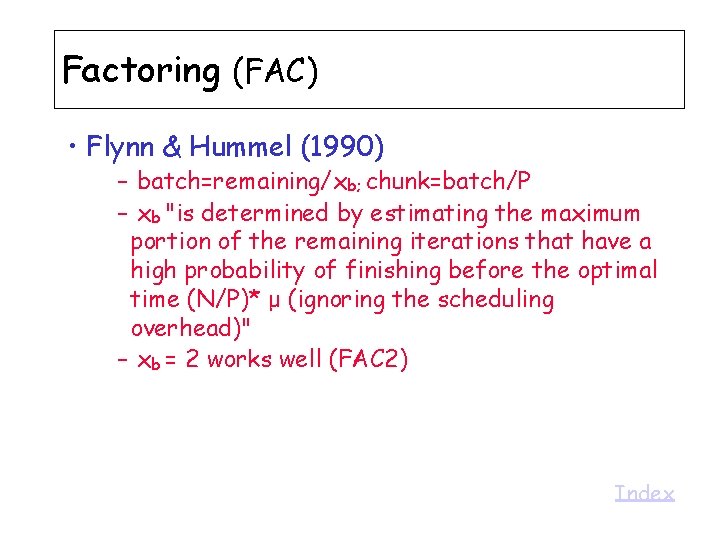
Factoring (FAC) • Flynn & Hummel (1990) – batch=remaining/xb; chunk=batch/P – xb "is determined by estimating the maximum portion of the remaining iterations that have a high probability of finishing before the optimal time (N/P)* μ (ignoring the scheduling overhead)" – xb = 2 works well (FAC 2) Index

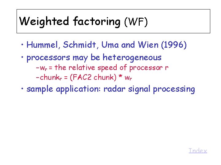
Weighted factoring (WF) • Hummel, Schmidt, Uma and Wien (1996) • processors may be heterogeneous – wr = the relative speed of processor r – chunkr = (FAC 2 chunk) * wr • sample application: radar signal processing Index

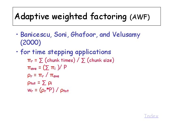
Adaptive weighted factoring (AWF) • Banicescu, Soni, Ghafoor, and Velusamy (2000) • for time stepping applications πr = ∑ (chunk times) / ∑ (chunk size) πave = (∑ πi )/ P ρr = πr / πave ρtot = ∑ ρi wr = (ρr*P) / ρtot Index

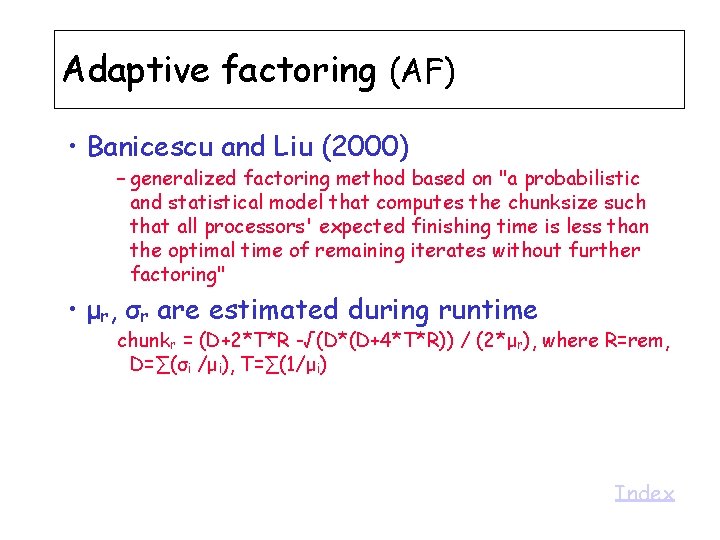
Adaptive factoring (AF) • Banicescu and Liu (2000) – generalized factoring method based on "a probabilistic and statistical model that computes the chunksize such that all processors' expected finishing time is less than the optimal time of remaining iterates without further factoring" • μr, σr are estimated during runtime chunkr = (D+2*T*R -√(D*(D+4*T*R)) / (2*μr), where R=rem, D=∑(σi /μi), T=∑(1/μi) Index

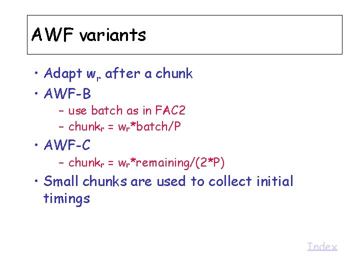
AWF variants • Adapt wr after a chunk • AWF-B – use batch as in FAC 2 – chunkr = wr*batch/P • AWF-C – chunkr = wr*remaining/(2*P) • Small chunks are used to collect initial timings Index

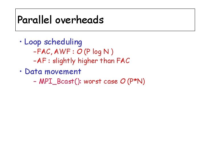
Parallel overheads • Loop scheduling – FAC, AWF : O (P log N ) – AF : slightly higher than FAC • Data movement – MPI_Bcast(): worst case O (P*N)