Automatic Performance Diagnosis of Parallel Computations with Compositional

Automatic Performance Diagnosis of Parallel Computations with Compositional Models Li Li, Allen D. Malony {lili, malony}@cs. uoregon. edu Performance Research Laboratory Dep. of Computer and Information Science University of Oregon

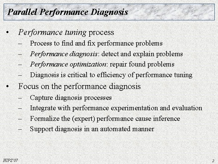
Parallel Performance Diagnosis • Performance tuning process – – • Focus on the performance diagnosis – – HIPS’ 07 Process to find and fix performance problems Performance diagnosis: detect and explain problems Performance optimization: repair found problems Diagnosis is critical to efficiency of performance tuning Capture diagnosis processes Integrate with performance experimentation and evaluation Formalize the (expert) performance cause inference Support diagnosis in an automated manner 2

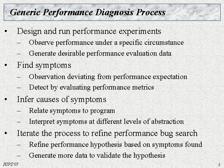
Generic Performance Diagnosis Process • Design and run performance experiments – – • Find symptoms – – • Observation deviating from performance expectation Detect by evaluating performance metrics Infer causes of symptoms – – • Observe performance under a specific circumstance Generate desirable performance evaluation data Relate symptoms to program Interpret symptoms at different levels of abstraction Iterate the process to refine performance bug search – – HIPS’ 07 Refine performance hypothesis based on symptoms found Generate more data to validate the hypothesis 3

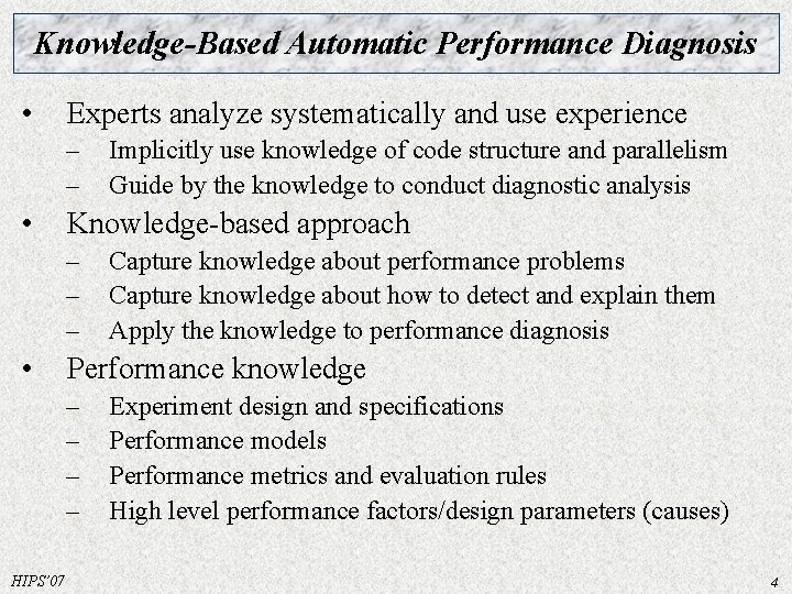
Knowledge-Based Automatic Performance Diagnosis • Experts analyze systematically and use experience – – • Knowledge-based approach – – – • Capture knowledge about performance problems Capture knowledge about how to detect and explain them Apply the knowledge to performance diagnosis Performance knowledge – – HIPS’ 07 Implicitly use knowledge of code structure and parallelism Guide by the knowledge to conduct diagnostic analysis Experiment design and specifications Performance models Performance metrics and evaluation rules High level performance factors/design parameters (causes) 4

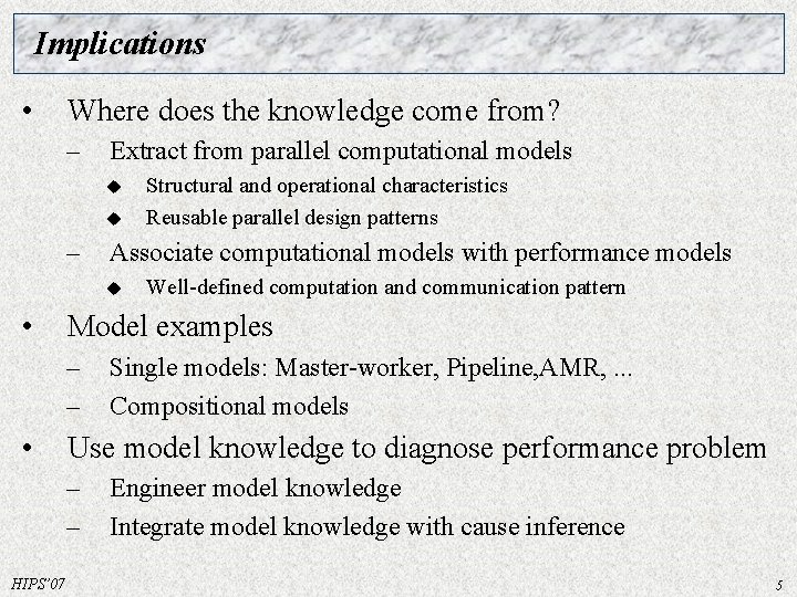
Implications • Where does the knowledge come from? – Extract from parallel computational models u u – Associate computational models with performance models u • Single models: Master-worker, Pipeline, AMR, . . . Compositional models Use model knowledge to diagnose performance problem – – HIPS’ 07 Well-defined computation and communication pattern Model examples – – • Structural and operational characteristics Reusable parallel design patterns Engineer model knowledge Integrate model knowledge with cause inference 5

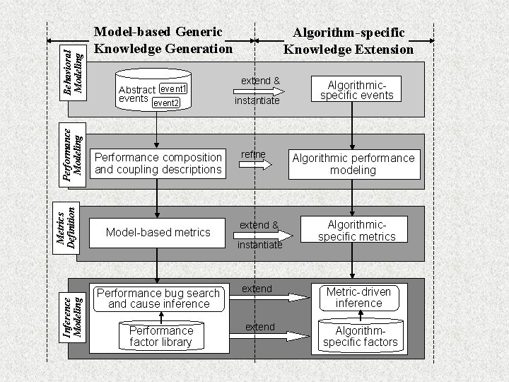
Behavioral Modeling Performance Modeling Metrics Definition Inference Modeling Model-based Generic Knowledge Generation Abstract event 1 events event 2 Performance composition and coupling descriptions Model-based metrics Algorithm-specific Knowledge Extension extend & instantiate refine extend & instantiate Performance bug search and cause inference Performance factor library extend Algorithmicspecific events Algorithmic performance modeling Algorithmicspecific metrics Metric-driven inference Algorithmspecific factors

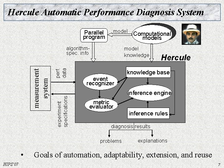
Hercule Automatic Performance Diagnosis System Parallel program model perf. data experiment specifications measurement system algorithmspec. info model knowledge event recognizer HIPS’ 07 Hercule knowledge base inference engine metric evaluator inference rules diagnosis results problems • Computational models explanations Goals of automation, adaptability, extension, and reuse 7

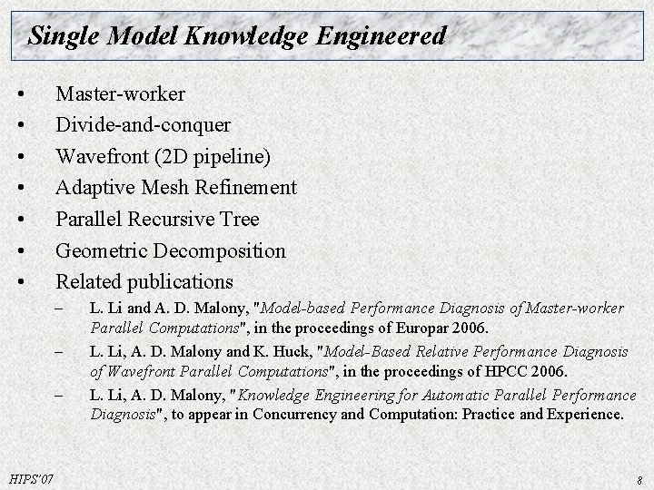
Single Model Knowledge Engineered • • Master-worker Divide-and-conquer Wavefront (2 D pipeline) Adaptive Mesh Refinement Parallel Recursive Tree Geometric Decomposition Related publications – – – HIPS’ 07 L. Li and A. D. Malony, "Model-based Performance Diagnosis of Master-worker Parallel Computations", in the proceedings of Europar 2006. L. Li, A. D. Malony and K. Huck, "Model-Based Relative Performance Diagnosis of Wavefront Parallel Computations", in the proceedings of HPCC 2006. L. Li, A. D. Malony, "Knowledge Engineering for Automatic Parallel Performance Diagnosis", to appear in Concurrency and Computation: Practice and Experience. 8

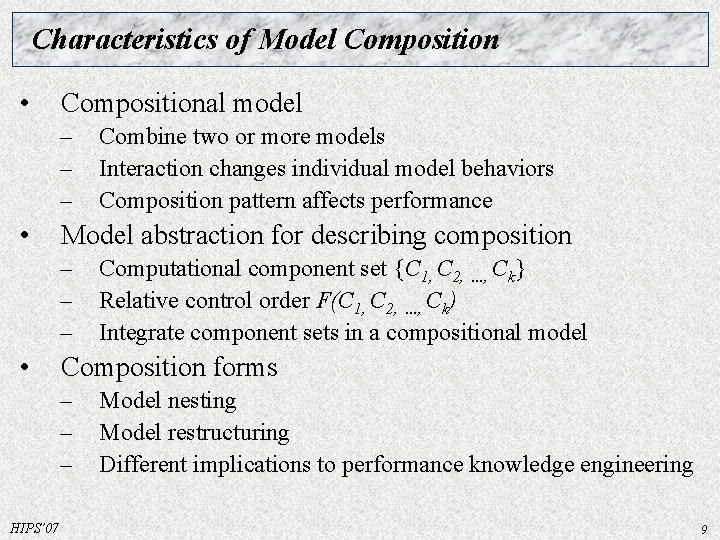
Characteristics of Model Composition • Compositional model – – – • Model abstraction for describing composition – – – • Computational component set {C 1, C 2, . . . , Ck} Relative control order F(C 1, C 2, . . . , Ck) Integrate component sets in a compositional model Composition forms – – – HIPS’ 07 Combine two or more models Interaction changes individual model behaviors Composition pattern affects performance Model nesting Model restructuring Different implications to performance knowledge engineering 9

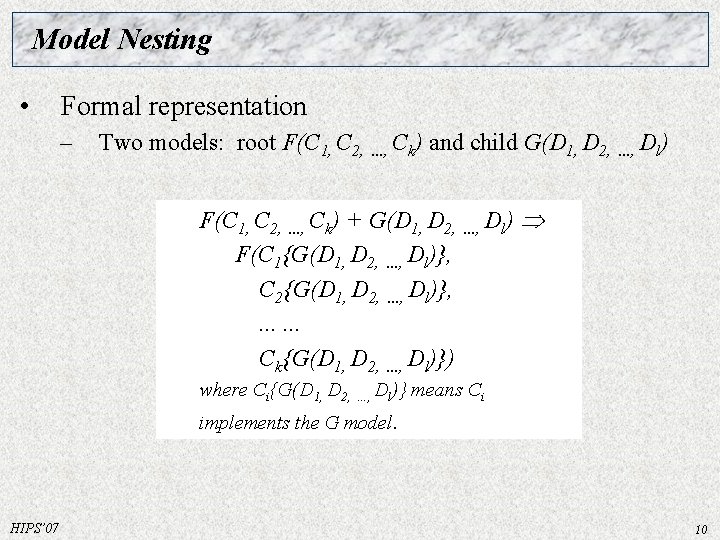
Model Nesting • Formal representation – Two models: root F(C 1, C 2, . . . , Ck) and child G(D 1, D 2, F(C 1, C 2, . . . , Ck) + G(D 1, D 2, F(C 1{G(D 1, D 2, . . . , Dl)}, C 2{G(D 1, D 2, . . . , Dl)}, . . . Ck{G(D 1, D 2, . . . , Dl)}) where Ci{G(D 1, D 2, . . . , Dl)} . . . , Dl) means Ci implements the G model. HIPS’ 07 10

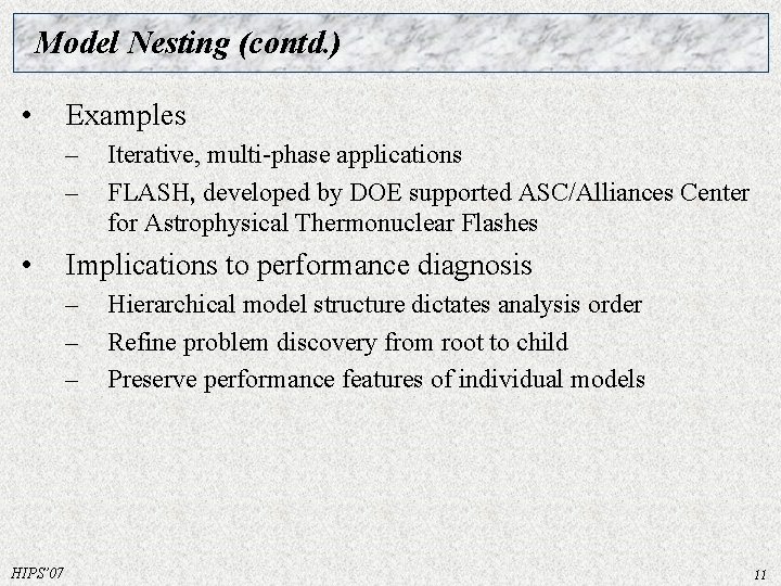
Model Nesting (contd. ) • Examples – – • Implications to performance diagnosis – – – HIPS’ 07 Iterative, multi-phase applications FLASH, developed by DOE supported ASC/Alliances Center for Astrophysical Thermonuclear Flashes Hierarchical model structure dictates analysis order Refine problem discovery from root to child Preserve performance features of individual models 11

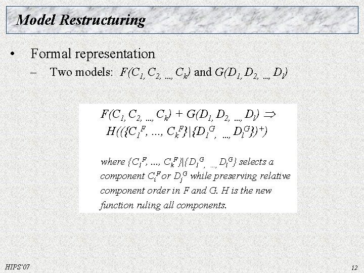
Model Restructuring • Formal representation – Two models: F(C 1, C 2, . . . , Ck) and G(D 1, D 2, . . . , Dl) F(C 1, C 2, . . . , Ck) + G(D 1, D 2, . . . , Dl) H(({C 1 F, . . . , Ck. F}|{D 1 G, . . . , Dl. G})+) where {C 1 F, . . . , Ck. F}|{D 1 G, . . . , Dl. G} selects a component Ci. F or Dj. G while preserving relative component order in F and G. H is the new function ruling all components. HIPS’ 07 12

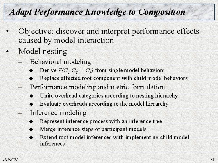
Adapt Performance Knowledge to Composition • • Objective: discover and interpret performance effects caused by model interaction Model nesting – Behavioral modeling u u – Performance modeling and metric formulation u u – Unite overhead categories according to nesting hierarchy Evaluate overheads according to the model hierarchy Inference modeling u u u HIPS’ 07 Derive F(C 1, C 2, . . . , Ck) from single model behaviors Replace affected root component with child model behaviors Represent inference process with an inference tree Merge inference steps of participant models Extend root model inferences with implementing child model inferences 13

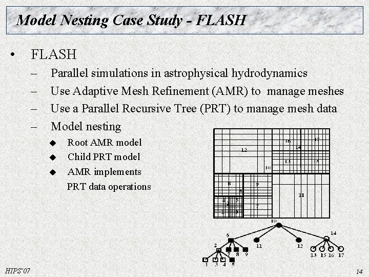
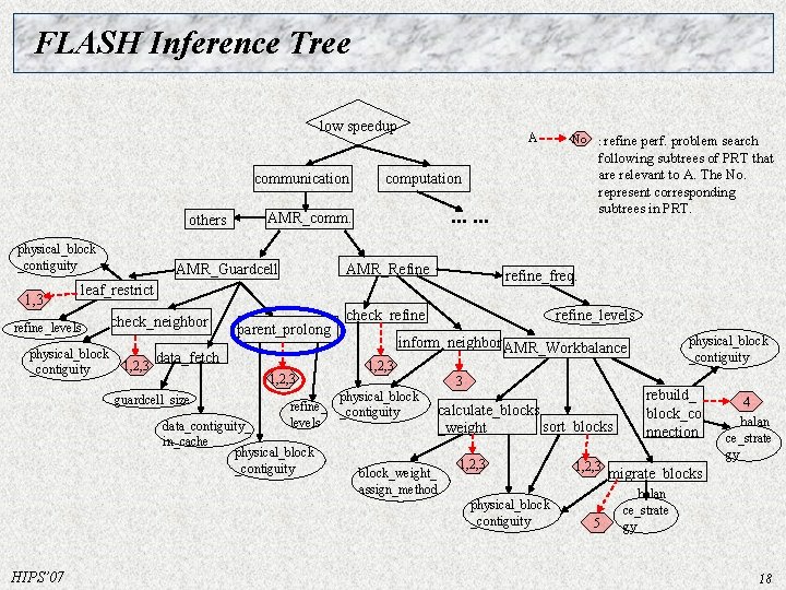
Model Nesting Case Study - FLASH • FLASH – – Parallel simulations in astrophysical hydrodynamics Use Adaptive Mesh Refinement (AMR) to manage meshes Use a Parallel Recursive Tree (PRT) to manage mesh data Model nesting u u u HIPS’ 07 Root AMR model Child PRT model AMR implements PRT data operations 14

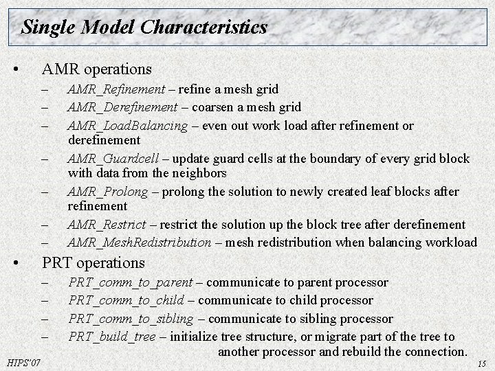
Single Model Characteristics • AMR operations – – – – • PRT operations – – HIPS’ 07 AMR_Refinement – refine a mesh grid AMR_Derefinement – coarsen a mesh grid AMR_Load. Balancing – even out work load after refinement or derefinement AMR_Guardcell – update guard cells at the boundary of every grid block with data from the neighbors AMR_Prolong – prolong the solution to newly created leaf blocks after refinement AMR_Restrict – restrict the solution up the block tree after derefinement AMR_Mesh. Redistribution – mesh redistribution when balancing workload PRT_comm_to_parent – communicate to parent processor PRT_comm_to_child – communicate to child processor PRT_comm_to_sibling – communicate to sibling processor PRT_build_tree – initialize tree structure, or migrate part of the tree to another processor and rebuild the connection. 15

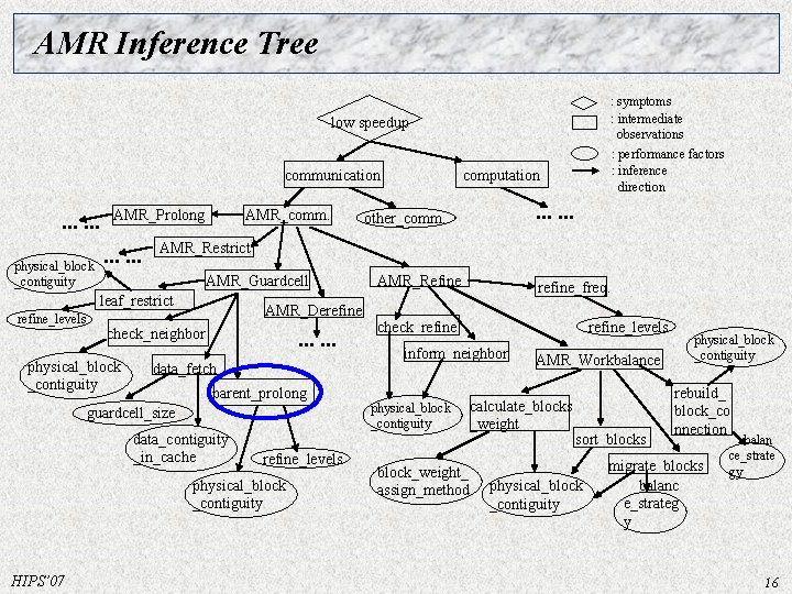
AMR Inference Tree : symptoms : intermediate observations : performance factors : inference direction low speedup communication . . . physical_block _contiguity AMR_Prolong . . . AMR_comm. AMR_Guardcell AMR_Derefine check_neighbor physical_block _contiguity . . . data_fetch parent_prolong guardcell_size data_contiguity _in_cache refine_levels physical_block _contiguity HIPS’ 07 . . . other_comm. AMR_Restrict leaf_restrict refine_levels computation AMR_Refine refine_freq. check_refine_levels inform_neighbor physical_block _contiguity block_weight_ assign_method AMR_Workbalance calculate_blocks _weight sort_blocks physical_block _contiguity rebuild_ block_co nnection migrate_blocks balanc e_strateg y balan ce_strate gy 16

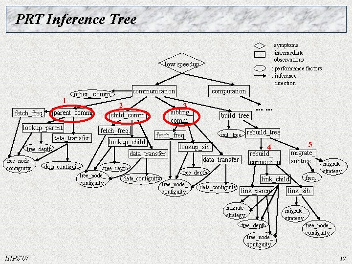
PRT Inference Tree : symptoms : intermediate observations : performance factors : inference direction low speedup 1 parent_comm fetch_freq. lookup_parent 2 tree_depth computation 3 sibling_ comm child_comm fetch_freq. data_transfer tree_node_ contiguity communication other_ comm lookup_child build_tree init. _tree rebuild_tree fetch_freq. data_transfer . . . 4 lookup_sib. rebuild_ connection data_transfer data_contiguity migrate_ subtree_depth tree_node_ freq. data_contiguity link_child contiguity tree_node_ data_contiguity link_parent link_sib. contiguity migrate_ strategy tree_depth tree_node_ contiguity HIPS’ 07 5 migrate_ strategy tree_node_ contiguity 17

FLASH Inference Tree low speedup communication others physical_block _contiguity 1, 3 A . . . AMR_Refine refine_freq. leaf_restrict refine_levels physical_block _contiguity check_neighbor data_fetch 1, 2, 3 guardcell_size parent_prolong 1, 2, 3 check_refine_levels 1, 2, 3 3 block_weight_ assign_method calculate_blocks sort_blocks _weight 1, 2, 3 physical_block _contiguity HIPS’ 07 physical_block _contiguity inform_neighbor AMR_Workbalance physical_block refine_ _contiguity levels data_contiguity_ in_cache physical_block _contiguity following subtrees of PRT that are relevant to A. The No. represent corresponding subtrees in PRT. computation AMR_comm. AMR_Guardcell No. : refine perf. problem search 1, 2, 3 5 rebuild_ block_co nnection 4 balan ce_strate gy migrate_blocks balan ce_strate gy 18

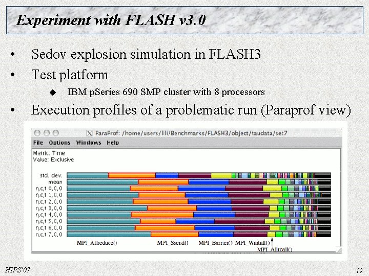
Experiment with FLASH v 3. 0 • • Sedov explosion simulation in FLASH 3 Test platform u • HIPS’ 07 IBM p. Series 690 SMP cluster with 8 processors Execution profiles of a problematic run (Paraprof view) 19

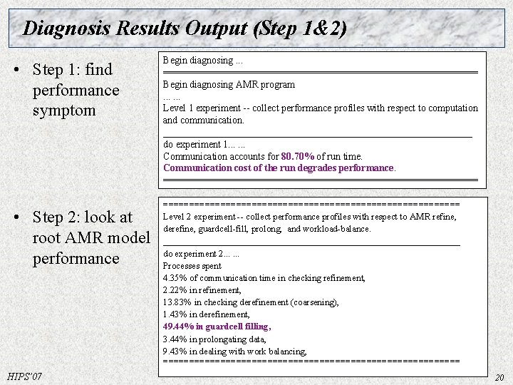
Diagnosis Results Output (Step 1&2) • Step 1: find performance symptom • Step 2: look at root AMR model performance HIPS’ 07 Begin diagnosing. . . ============================ Begin diagnosing AMR program. . . Level 1 experiment -- collect performance profiles with respect to computation and communication. _______________________________ do experiment 1. . . Communication accounts for 80. 70% of run time. Communication cost of the run degrades performance. ========================================================= Level 2 experiment -- collect performance profiles with respect to AMR refine, derefine, guardcell-fill, prolong, and workload-balance. ________________________________ do experiment 2. . . Processes spent 4. 35% of communication time in checking refinement, 2. 22% in refinement, 13. 83% in checking derefinement (coarsening), 1. 43% in derefinement, 49. 44% in guardcell filling, 3. 44% in prolongating data, 9. 43% in dealing with work balancing, ============================= 20

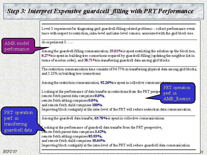
Step 3: Interpret Expensive guardcell_filling with PRT Performance ================================== AMR model performance Level 3 experiment for diagnosing grid guardcell-filling related problems -- collect performance event trace with respect to restriction, intra-level and inter-level commu. associated with the grid block tree. __________________________________________ do experiment 3. . . Among the guardcell-filling communication, 53. 01% is spent restricting the solution up the block tree, 8. 27% is spent in building tree connections required by guardcell-filling (updating the neighbor list in terms of morton order), and 38. 71% in transferring guardcell data among grid blocks. __________________________________________ The restriction communication time consists of 94. 77% in transferring physical data among grid blocks, and 5. 23% in building tree connections. Among the restriction communication, 92. 26% is spent in collective communications. PRT operation perf. in transferring guardcell data HIPS’ 07 Looking at the performance of data transfer in restrictions from the PRT perspective, perf. in remote fetch parent data comprises 0. 0%, AMR_Restrict remote fetch sibling comprises 0. 0%, and remote fetch child comprises 100%. Improving block contiguity at the inter-level of the PRT will reduce restriction data communication. _________________________________________ Among the guardcell data transfer, 65. 78% is spent in collective communications. Looking at the performance of guardcell data transfer from the PRT perspective, remote fetch parent data comprises 3. 42%, remote fetch sibling comprises 85. 93%, and remote fetch child comprises 10. 64%. Improving block contiguity at the intra-level of the PRT will reduce guardcell data communication. ================================== 21

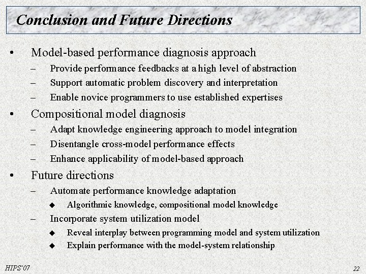
Conclusion and Future Directions • Model-based performance diagnosis approach – – – • Compositional model diagnosis – – – • Provide performance feedbacks at a high level of abstraction Support automatic problem discovery and interpretation Enable novice programmers to use established expertises Adapt knowledge engineering approach to model integration Disentangle cross-model performance effects Enhance applicability of model-based approach Future directions – Automate performance knowledge adaptation u – Incorporate system utilization model u u HIPS’ 07 Algorithmic knowledge, compositional model knowledge Reveal interplay between programming model and system utilization Explain performance with the model-system relationship 22