Automatic Lung Nodule Detection Using Deep Learning and

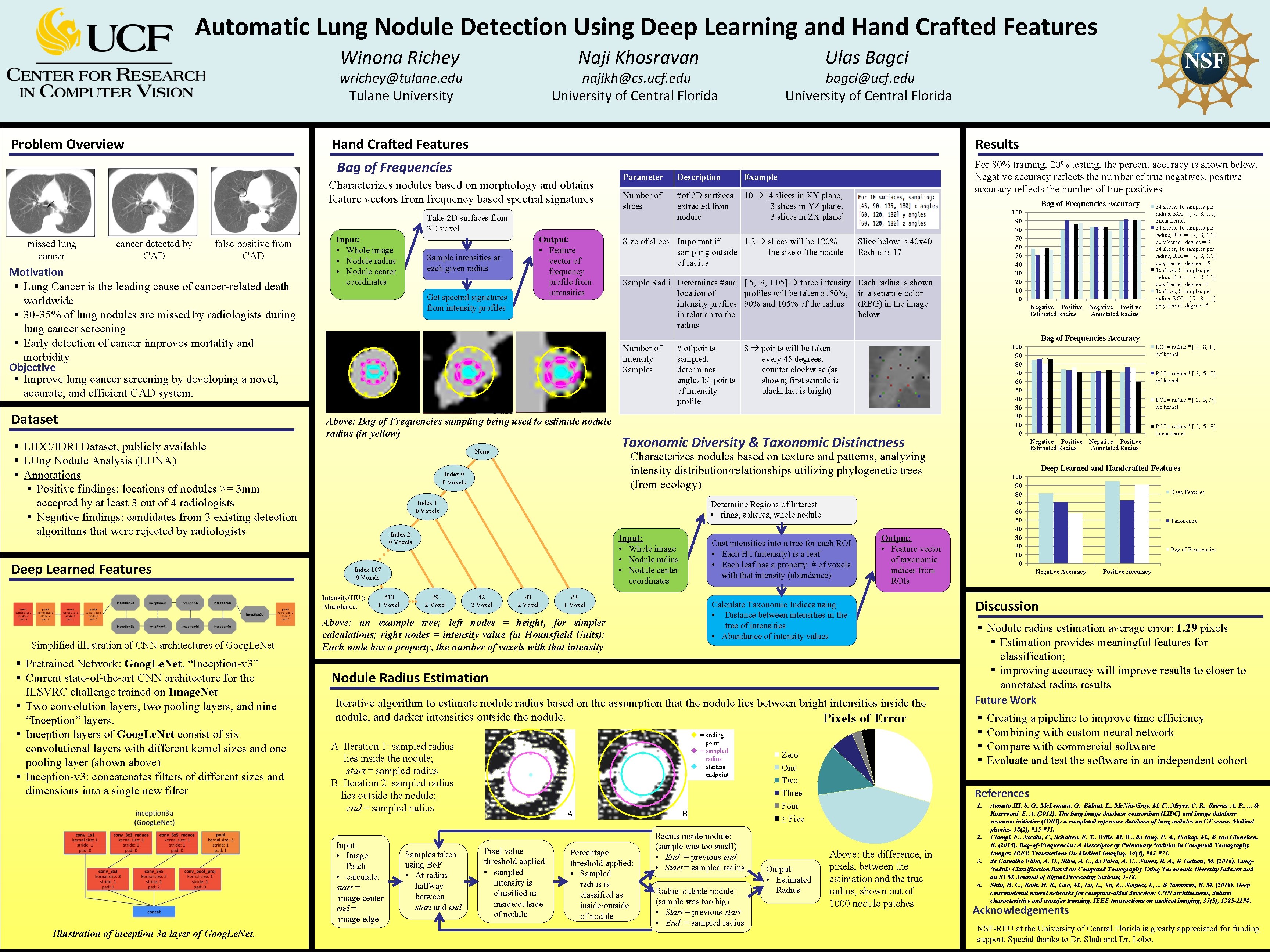
Automatic Lung Nodule Detection Using Deep Learning and Hand Crafted Features Winona Richey Naji Khosravan wrichey@tulane. edu Tulane University Problem Overview najikh@cs. ucf. edu University of Central Florida Results Characterizes nodules based on morphology and obtains feature vectors from frequency based spectral signatures Parameter Description Example Number of slices #of 2 D surfaces extracted from nodule 10 [4 slices in XY plane, 3 slices in YZ plane, 3 slices in ZX plane] Take 2 D surfaces from 3 D voxel cancer detected by CAD bagci@ucf. edu University of Central Florida Hand Crafted Features Bag of Frequencies missed lung cancer Ulas Bagci false positive from CAD Motivation § Lung Cancer is the leading cause of cancer-related death worldwide § 30 -35% of lung nodules are missed by radiologists during lung cancer screening § Early detection of cancer improves mortality and morbidity Objective § Improve lung cancer screening by developing a novel, accurate, and efficient CAD system. Dataset Input: • Whole image • Nodule radius • Nodule center coordinates § Pretrained Network: Goog. Le. Net, “Inception-v 3” § Current state-of-the-art CNN architecture for the ILSVRC challenge trained on Image. Net § Two convolution layers, two pooling layers, and nine “Inception” layers. § Inception layers of Goog. Le. Net consist of six convolutional layers with different kernel sizes and one pooling layer (shown above) § Inception-v 3: concatenates filters of different sizes and dimensions into a single new filter Size of slices Important if 1. 2 slices will be 120% sampling outside the size of the nodule of radius Slice below is 40 x 40 Radius is 17 Sample Radii Determines #and [. 5, . 9, 1. 05] three intensity location of profiles will be taken at 50%, intensity profiles 90% and 105% of the radius in relation to the radius Each radius is shown in a separate color (RBG) in the image below Number of intensity Samples Above: Bag of Frequencies sampling being used to estimate nodule radius (in yellow) None 100 90 80 70 60 50 40 30 20 10 0 Negative Positive Estimated Radius # of points sampled; determines angles b/t points of intensity profile Negative Positive Annotated Radius Taxonomic Diversity & Taxonomic Distinctness Index 1 0 Voxels 34 slices, 16 samples per radius, ROI = [. 7, . 8, 1. 1], linear kernel 34 slices, 16 samples per radius, ROI = [. 7, . 8, 1. 1], poly kernel, degree = 3 34 slices, 16 samples per radius, ROI = [. 7, . 8, 1. 1], poly kernel, degree = 5 16 slices, 8 samples per radius, ROI = [. 7, . 8, 1. 1], poly kernel, degree =3 16 slices, 8 samples per radius, ROI = [. 7, . 8, 1. 1], poly kernel, degree =5 Input: • Whole image • Nodule radius • Nodule center coordinates Index 107 0 Voxels 29 2 Voxel 42 2 Voxel 43 2 Voxel Cast intensities into a tree for each ROI • Each HU(intensity) is a leaf • Each leaf has a property: # of voxels with that intensity (abundance) 63 1 Voxel Above: an example tree; left nodes = height, for simpler calculations; right nodes = intensity value (in Hounsfield Units); Each node has a property, the number of voxels with that intensity Nodule Radius Estimation Iterative algorithm to estimate nodule radius based on the assumption that the nodule lies between bright intensities inside the nodule, and darker intensities outside the nodule. Pixels of Error u = ending point u = sampled radius u = starting endpoint A. Iteration 1: sampled radius lies inside the nodule; start = sampled radius B. Iteration 2: sampled radius lies outside the nodule; end = sampled radius Samples taken using Bo. F • At radius halfway between start and end A Pixel value threshold applied: • sampled intensity is classified as inside/outside of nodule Percentage threshold applied: • Sampled radius is classified as inside/outside of nodule B Radius inside nodule: (sample was too small) • End = previous end • Start = sampled radius Radius outside nodule: (sample was too big) • Start = previous start • End = sampled radius Zero One Two Three Four ≥ Five ROI = radius * [. 2, . 5, . 7], rbf kernel ROI = radius * [. 3, . 5, . 8], linear kernel Negative Positive Annotated Radius 100 90 80 70 60 50 40 30 20 10 0 Deep Features Taxonomic Bag of Frequencies Negative Accuracy Positive Accuracy Discussion § Nodule radius estimation average error: 1. 29 pixels § Estimation provides meaningful features for classification; § improving accuracy will improve results to closer to annotated radius results Future Work § § Creating a pipeline to improve time efficiency Combining with custom neural network Compare with commercial software Evaluate and test the software in an independent cohort References 1. 2. Output: • Estimated Radius ROI = radius * [. 3, . 5, . 8], rbf kernel Deep Learned and Handcrafted Features Output: • Feature vector of taxonomic indices from ROIs Calculate Taxonomic Indices using • Distance between intensities in the tree of intensities • Abundance of intensity values ROI = radius * [. 5, . 8, 1], rbf kernel Negative Positive Estimated Radius Determine Regions of Interest • rings, spheres, whole nodule Index 2 0 Voxels -513 1 Voxel 100 90 80 70 60 50 40 30 20 10 0 8 points will be taken every 45 degrees, counter clockwise (as shown; first sample is black, last is bright) Characterizes nodules based on texture and patterns, analyzing intensity distribution/relationships utilizing phylogenetic trees (from ecology) Index 0 0 Voxels Input: • Image Patch • calculate: start = image center end = image edge Illustration of inception 3 a layer of Goog. Le. Net. Bag of Frequencies Accuracy Intensity(HU): Abundance: Simplified illustration of CNN architectures of Goog. Le. Net Sample intensities at each given radius Get spectral signatures from intensity profiles § LIDC/IDRI Dataset, publicly available § LUng Nodule Analysis (LUNA) § Annotations § Positive findings: locations of nodules >= 3 mm accepted by at least 3 out of 4 radiologists § Negative findings: candidates from 3 existing detection algorithms that were rejected by radiologists Deep Learned Features Output: • Feature vector of frequency profile from intensities For 80% training, 20% testing, the percent accuracy is shown below. Negative accuracy reflects the number of true negatives, positive accuracy reflects the number of true positives Above: the difference, in pixels, between the estimation and the true radius; shown out of 1000 nodule patches 3. 4. Armato III, S. G. , Mc. Lennan, G. , Bidaut, L. , Mc. Nitt-Gray, M. F. , Meyer, C. R. , Reeves, A. P. , . . . & Kazerooni, E. A. (2011). The lung image database consortium (LIDC) and image database resource initiative (IDRI): a completed reference database of lung nodules on CT scans. Medical physics, 38(2), 915 -931. Ciompi, F. , Jacobs, C. , Scholten, E. T. , Wille, M. W. , de Jong, P. A. , Prokop, M. , & van Ginneken, B. (2015). Bag-of-Frequencies: A Descriptor of Pulmonary Nodules in Computed Tomography Images. IEEE Transactions On Medical Imaging, 34(4), 962 -973. de Carvalho Filho, A. O. , Silva, A. C. , de Paiva, A. C. , Nunes, R. A. , & Gattass, M. (2016). Lung. Nodule Classification Based on Computed Tomography Using Taxonomic Diversity Indexes and an SVM. Journal of Signal Processing Systems, 1 -18. Shin, H. C. , Roth, H. R. , Gao, M. , Lu, L. , Xu, Z. , Nogues, I. , . . . & Summers, R. M. (2016). Deep convolutional neural networks for computer-aided detection: CNN architectures, dataset characteristics and transfer learning. IEEE transactions on medical imaging, 35(5), 1285 -1298. Acknowledgements NSF-REU at the University of Central Florida is greatly appreciated for funding support. Special thanks to Dr. Shah and Dr. Lobo.