Automatic Differentiation Tutorial Paul Hovland Andrew Lyons Boyana

Automatic Differentiation Tutorial Paul Hovland Andrew Lyons Boyana Norris Jean Utke Mathematics & Computer Science Division Argonne National Laboratory

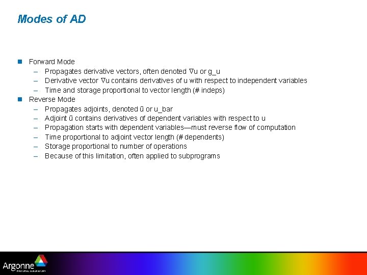
Modes of AD n Forward Mode – Propagates derivative vectors, often denoted u or g_u – Derivative vector u contains derivatives of u with respect to independent variables – Time and storage proportional to vector length (# indeps) n Reverse Mode – Propagates adjoints, denoted ū or u_bar – Adjoint ū contains derivatives of dependent variables with respect to u – Propagation starts with dependent variables—must reverse flow of computation – Time proportional to adjoint vector length (# dependents) – Storage proportional to number of operations – Because of this limitation, often applied to subprograms

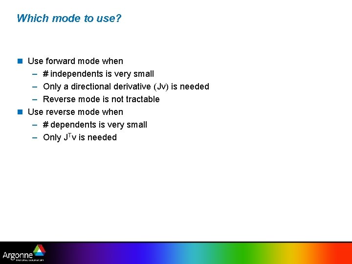
Which mode to use? n Use forward mode when – # independents is very small – Only a directional derivative (Jv) is needed – Reverse mode is not tractable n Use reverse mode when – # dependents is very small – Only JTv is needed

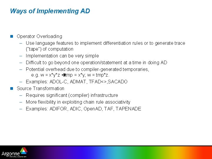
Ways of Implementing AD n Operator Overloading – Use language features to implement differentiation rules or to generate trace (“tape”) of computation – Implementation can be very simple – Difficult to go beyond one operation/statement at a time in doing AD – Potential overhead due to compiler-generated temporaries, e. g. w = x*y*z ètmp = x*y; w = tmp*z. – Examples: ADOL-C, ADMAT, TFAD<>, SACADO n Source Transformation – Requires significant (compiler) infrastructure – More flexibility in exploiting chain rule associativity – Examples: ADIFOR, ADIC, Open. AD, TAF, TAPENADE

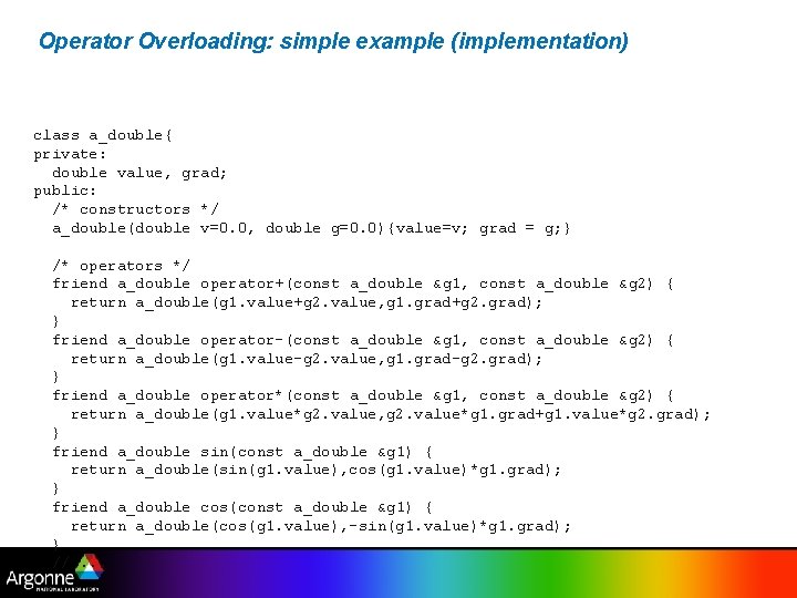
Operator Overloading: simple example (implementation) class a_double{ private: double value, grad; public: /* constructors */ a_double(double v=0. 0, double g=0. 0){value=v; grad = g; } /* operators */ friend a_double operator+(const a_double &g 1, const a_double &g 2) { return a_double(g 1. value+g 2. value, g 1. grad+g 2. grad); } friend a_double operator-(const a_double &g 1, const a_double &g 2) { return a_double(g 1. value-g 2. value, g 1. grad-g 2. grad); } friend a_double operator*(const a_double &g 1, const a_double &g 2) { return a_double(g 1. value*g 2. value, g 2. value*g 1. grad+g 1. value*g 2. grad); } friend a_double sin(const a_double &g 1) { return a_double(sin(g 1. value), cos(g 1. value)*g 1. grad); } friend a_double cos(const a_double &g 1) { return a_double(cos(g 1. value), -sin(g 1. value)*g 1. grad); } //. . .

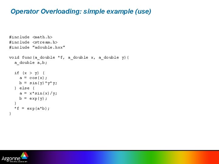
Operator Overloading: simple example (use) #include <math. h> #include <stream. h> #include "adouble. hxx" void func(a_double *f, a_double x, a_double y){ a_double a, b; if (x > y) { a = cos(x); b = sin(y)*y*y; } else { a = x*sin(x)/y; b = exp(y); } *f = exp(a*b); }

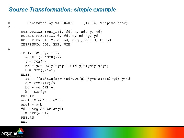
Source Transformation: simple example C C Generated by TAPENADE (INRIA, Tropics team) . . . SUBROUTINE FUNC_D(f, fd, x, xd, y, yd) DOUBLE PRECISION f, fd, x, xd, y, yd DOUBLE PRECISION a, ad, arg 1 d, b, bd INTRINSIC COS, EXP, SIN C IF (x. GT. y) THEN ad = -(xd*SIN(x)) a = COS(x) bd = yd*COS(y)*y*y + SIN(y)*(yd*y+y*yd) b = SIN(y)*y*y ELSE ad = ((xd*SIN(x)+x*xd*COS(x))*y-x*SIN(x)*yd)/y**2 a = x*SIN(x)/y bd = yd*EXP(y) b = EXP(y) END IF arg 1 d = ad*b + a*bd arg 1 = a*b fd = arg 1 d*EXP(arg 1) f = EXP(arg 1) RETURN END

Tools n n n Fortran 95 C/C++ Fortran 77 MATLAB Other languages: Ada, Python, . . . More tools at http: //www. autodiff. org/

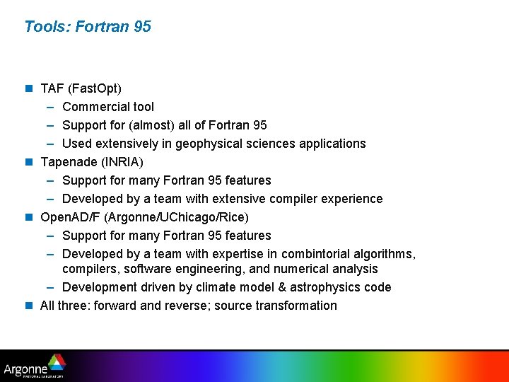
Tools: Fortran 95 n TAF (Fast. Opt) – Commercial tool – Support for (almost) all of Fortran 95 – Used extensively in geophysical sciences applications n Tapenade (INRIA) – Support for many Fortran 95 features – Developed by a team with extensive compiler experience n Open. AD/F (Argonne/UChicago/Rice) – Support for many Fortran 95 features – Developed by a team with expertise in combintorial algorithms, compilers, software engineering, and numerical analysis – Development driven by climate model & astrophysics code n All three: forward and reverse; source transformation

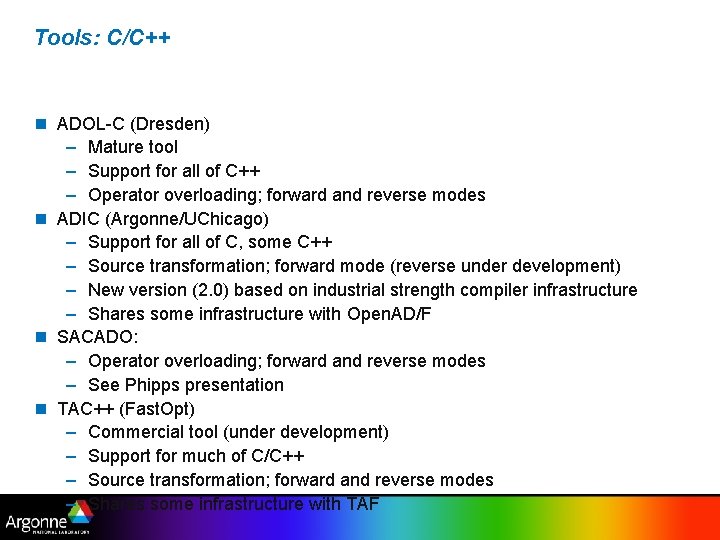
Tools: C/C++ n ADOL-C (Dresden) – Mature tool – Support for all of C++ – Operator overloading; forward and reverse modes n ADIC (Argonne/UChicago) – Support for all of C, some C++ – Source transformation; forward mode (reverse under development) – New version (2. 0) based on industrial strength compiler infrastructure – Shares some infrastructure with Open. AD/F n SACADO: – Operator overloading; forward and reverse modes – See Phipps presentation n TAC++ (Fast. Opt) – Commercial tool (under development) – Support for much of C/C++ – Source transformation; forward and reverse modes – Shares some infrastructure with TAF

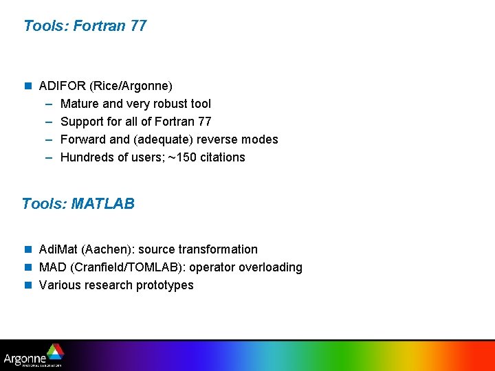
Tools: Fortran 77 n ADIFOR (Rice/Argonne) – Mature and very robust tool – Support for all of Fortran 77 – Forward and (adequate) reverse modes – Hundreds of users; ~150 citations Tools: MATLAB n Adi. Mat (Aachen): source transformation n MAD (Cranfield/TOMLAB): operator overloading n Various research prototypes

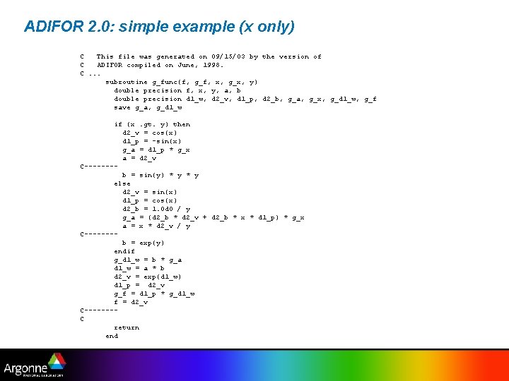
ADIFOR 2. 0: simple example (x only) C This file was generated on 09/15/03 by the version of C ADIFOR compiled on June, 1998. C. . . subroutine g_func(f, g_f, x, g_x, y) double precision f, x, y, a, b double precision d 1_w, d 2_v, d 1_p, d 2_b, g_a, g_x, g_d 1_w, g_f save g_a, g_d 1_w if (x. gt. y) then d 2_v = cos(x) d 1_p = -sin(x) g_a = d 1_p * g_x a = d 2_v C-------b = sin(y) * y else d 2_v = sin(x) d 1_p = cos(x) d 2_b = 1. 0 d 0 / y g_a = (d 2_b * d 2_v + d 2_b * x * d 1_p) * g_x a = x * d 2_v / y C-------b = exp(y) endif g_d 1_w = b * g_a d 1_w = a * b d 2_v = exp(d 1_w) d 1_p = d 2_v g_f = d 1_p * g_d 1_w f = d 2_v C-------C return end

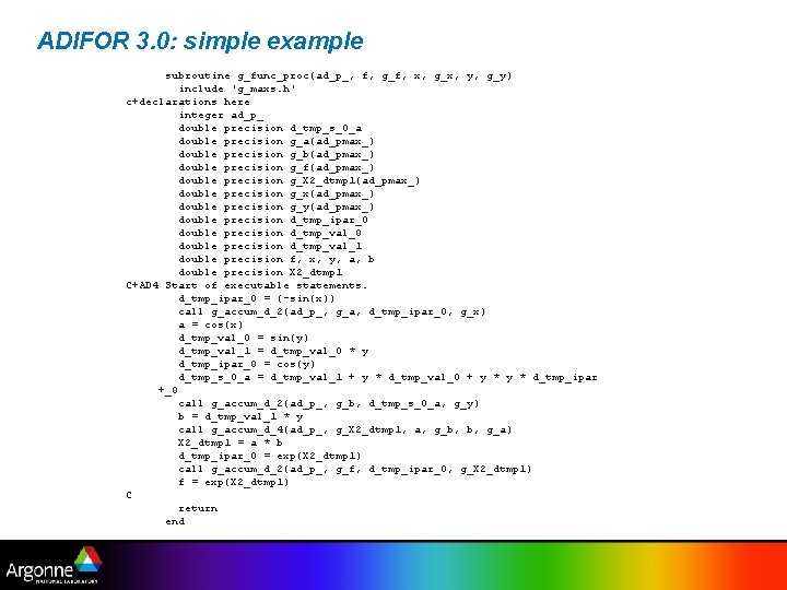
ADIFOR 3. 0: simple example subroutine g_func_proc(ad_p_, f, g_f, x, g_x, y, g_y) include 'g_maxs. h' c+declarations here integer ad_p_ double precision d_tmp_s_0_a double precision g_a(ad_pmax_) double precision g_b(ad_pmax_) double precision g_f(ad_pmax_) double precision g_X 2_dtmp 1(ad_pmax_) double precision g_x(ad_pmax_) double precision g_y(ad_pmax_) double precision d_tmp_ipar_0 double precision d_tmp_val_1 double precision f, x, y, a, b double precision X 2_dtmp 1 C+AD 4 Start of executable statements. d_tmp_ipar_0 = (-sin(x)) call g_accum_d_2(ad_p_, g_a, d_tmp_ipar_0, g_x) a = cos(x) d_tmp_val_0 = sin(y) d_tmp_val_1 = d_tmp_val_0 * y d_tmp_ipar_0 = cos(y) d_tmp_s_0_a = d_tmp_val_1 + y * d_tmp_val_0 + y * d_tmp_ipar +_0 call g_accum_d_2(ad_p_, g_b, d_tmp_s_0_a, g_y) b = d_tmp_val_1 * y call g_accum_d_4(ad_p_, g_X 2_dtmp 1, a, g_b, b, g_a) X 2_dtmp 1 = a * b d_tmp_ipar_0 = exp(X 2_dtmp 1) call g_accum_d_2(ad_p_, g_f, d_tmp_ipar_0, g_X 2_dtmp 1) f = exp(X 2_dtmp 1) C return end

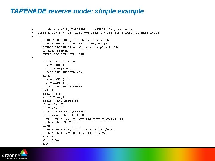
TAPENADE reverse mode: simple example C Generated by TAPENADE (INRIA, Tropics team) C Version 2. 0. 6 - (Id: 1. 14 vmp Stable - Fri Sep 5 14: 08: 23 MEST 2003) C. . . SUBROUTINE FUNC_B(f, fb, x, xb, y, yb) DOUBLE PRECISION f, fb, x, xb, y, yb DOUBLE PRECISION a, ab, arg 1 b, b, bb INTEGER branch INTRINSIC COS, EXP, SIN C IF (x. GT. y) THEN a = COS(x) b = SIN(y)*y*y CALL PUSHINTEGER 4(0) ELSE a = x*SIN(x)/y b = EXP(y) CALL PUSHINTEGER 4(1) END IF arg 1 = a*b f = EXP(arg 1) arg 1 b = EXP(arg 1)*fb ab = b*arg 1 b bb = a*arg 1 b CALL POPINTEGER 4(branch) IF (branch. LT. 1) THEN yb = yb + (SIN(y)*y+y*SIN(y)+y*y*COS(y))*bb xb = xb - SIN(x)*ab ELSE yb = yb + EXP(y)*bb - x*SIN(x)*ab/y**2 xb = xb + (x*COS(x)/y+SIN(x)/y)*ab END IF fb = 0. D 0 END

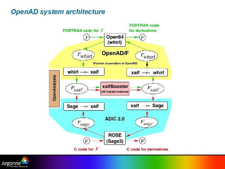
Open. AD system architecture

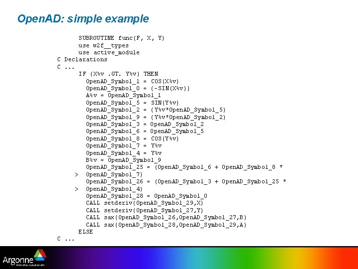
Open. AD: simple example SUBROUTINE func(F, X, Y) use w 2 f__types use active_module C Declarations C. . . IF (X%v. GT. Y%v) THEN Open. AD_Symbol_1 = COS(X%v) Open. AD_Symbol_0 = (- SIN(X%v)) A%v = Open. AD_Symbol_1 Open. AD_Symbol_5 = SIN(Y%v) Open. AD_Symbol_2 = ( Y%v*Open. AD_Symbol_5) Open. AD_Symbol_9 = ( Y%v*Open. AD_Symbol_2) Open. AD_Symbol_3 = Open. AD_Symbol_2 Open. AD_Symbol_6 = Open. AD_Symbol_5 Open. AD_Symbol_8 = COS(Y%v) Open. AD_Symbol_7 = Y%v Open. AD_Symbol_4 = Y%v B%v = Open. AD_Symbol_9 Open. AD_Symbol_25 = (Open. AD_Symbol_6 + Open. AD_Symbol_8 * > Open. AD_Symbol_7) Open. AD_Symbol_26 = (Open. AD_Symbol_3 + Open. AD_Symbol_25 * > Open. AD_Symbol_4) Open. AD_Symbol_28 = Open. AD_Symbol_0 CALL setderiv(Open. AD_Symbol_29, X) CALL setderiv(Open. AD_Symbol_27, Y) CALL sax(Open. AD_Symbol_26, Open. AD_Symbol_27, B) CALL sax(Open. AD_Symbol_28, Open. AD_Symbol_29, A) ELSE C. . .

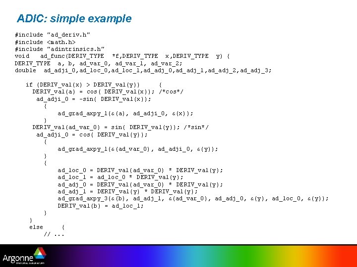
ADIC: simple example #include "ad_deriv. h" #include <math. h> #include "adintrinsics. h" void ad_func(DERIV_TYPE *f, DERIV_TYPE x, DERIV_TYPE y) { DERIV_TYPE a, b, ad_var_0, ad_var_1, ad_var_2; double ad_adji_0, ad_loc_1, ad_adj_0, ad_adj_1, ad_adj_2, ad_adj_3; if (DERIV_val(x) > DERIV_val(y)) { DERIV_val(a) = cos( DERIV_val(x)); /*cos*/ ad_adji_0 = -sin( DERIV_val(x)); { ad_grad_axpy_1(&(a), ad_adji_0, &(x)); } DERIV_val(ad_var_0) = sin( DERIV_val(y)); /*sin*/ ad_adji_0 = cos( DERIV_val(y)); { ad_grad_axpy_1(&(ad_var_0), ad_adji_0, &(y)); } { ad_loc_0 = DERIV_val(ad_var_0) * DERIV_val(y); ad_loc_1 = ad_loc_0 * DERIV_val(y); ad_adj_0 = DERIV_val(ad_var_0) * DERIV_val(y); ad_adj_1 = DERIV_val(y) * DERIV_val(y); ad_grad_axpy_3(&(b), ad_adj_1, &(ad_var_0), ad_adj_0, &(y), ad_loc_0, &(y)); DERIV_val(b) = ad_loc_1; } } else { //. . .

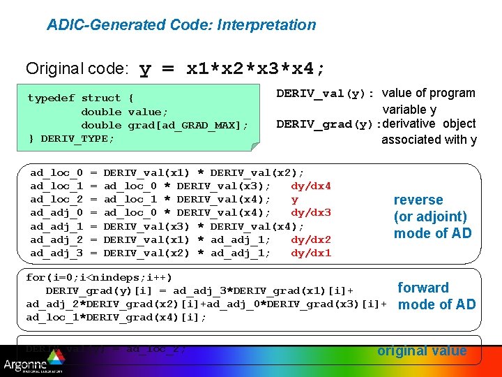
ADIC-Generated Code: Interpretation Original code: y = x 1*x 2*x 3*x 4; typedef struct { double value; double grad[ad_GRAD_MAX]; } DERIV_TYPE; ad_loc_0 ad_loc_1 ad_loc_2 ad_adj_0 ad_adj_1 ad_adj_2 ad_adj_3 = = = = DERIV_val(y): value of program variable y DERIV_grad(y): derivative object associated with y DERIV_val(x 1) * DERIV_val(x 2); ad_loc_0 * DERIV_val(x 3); dy/dx 4 ad_loc_1 * DERIV_val(x 4); y ad_loc_0 * DERIV_val(x 4); dy/dx 3 DERIV_val(x 3) * DERIV_val(x 4); DERIV_val(x 1) * ad_adj_1; dy/dx 2 DERIV_val(x 2) * ad_adj_1; dy/dx 1 reverse (or adjoint) mode of AD for(i=0; i<nindeps; i++) DERIV_grad(y)[i] = ad_adj_3*DERIV_grad(x 1)[i]+ ad_adj_2*DERIV_grad(x 2)[i]+ad_adj_0*DERIV_grad(x 3)[i]+ ad_loc_1*DERIV_grad(x 4)[i]; DERIV_val(y) = ad_loc_2; forward mode of AD original value

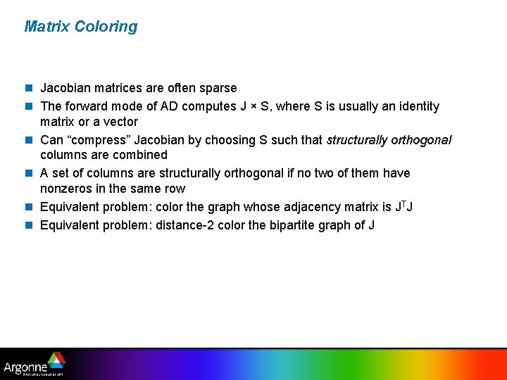
Matrix Coloring n Jacobian matrices are often sparse n The forward mode of AD computes J × S, where S is usually an identity matrix or a vector n Can “compress” Jacobian by choosing S such that structurally orthogonal columns are combined n A set of columns are structurally orthogonal if no two of them have nonzeros in the same row n Equivalent problem: color the graph whose adjacency matrix is JTJ n Equivalent problem: distance-2 color the bipartite graph of J

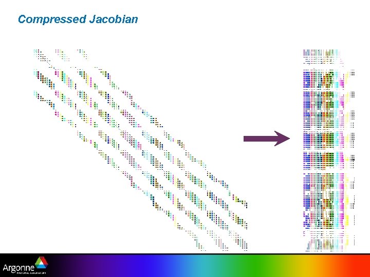
Compressed Jacobian

What is feasible & practical n Key point: forward mode computes JS at cost proportional to number of columns in S; reverse mode computes JTW at cost proportional to number of columns in W n Jacobians of functions with small number (1— 1000) of independent variables (forward mode, S=I) n Jacobians of functions with small number (1— 100) of dependent variables (reverse/adjoint mode, S=I) n Very (extremely) large, but (very) sparse Jacobians and Hessians (forward mode plus coloring) n Jacobian-vector products (forward mode) n Transposed-Jacobian-vector products (adjoint mode) n Hessian-vector products (forward + adjoint modes) n Large, dense Jacobian matrices that are effectively sparse or effectively low rank (e. g. , see Abdel-Khalik et al. , AD 2008)

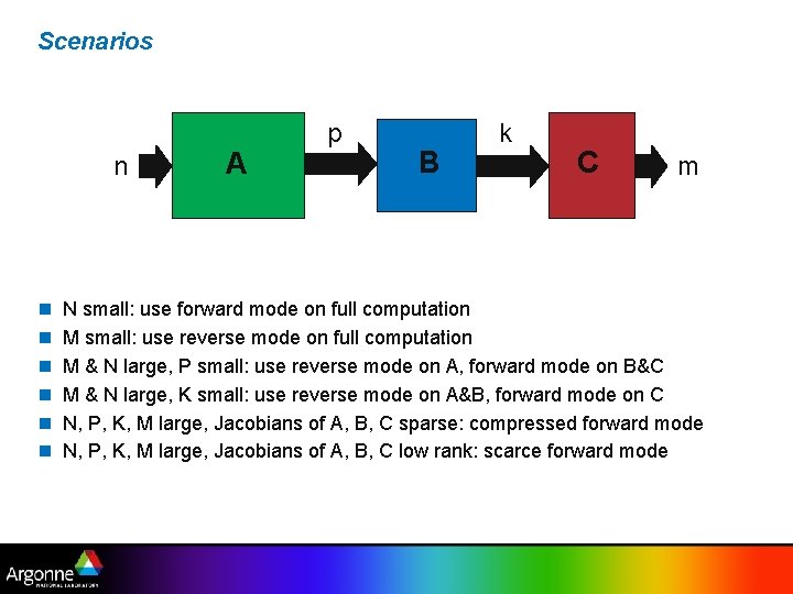
Scenarios n n n n A p B k C m N small: use forward mode on full computation M small: use reverse mode on full computation M & N large, P small: use reverse mode on A, forward mode on B&C M & N large, K small: use reverse mode on A&B, forward mode on C N, P, K, M large, Jacobians of A, B, C sparse: compressed forward mode N, P, K, M large, Jacobians of A, B, C low rank: scarce forward mode

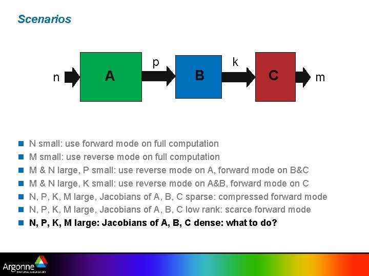
Scenarios n n n n A p B k C m N small: use forward mode on full computation M small: use reverse mode on full computation M & N large, P small: use reverse mode on A, forward mode on B&C M & N large, K small: use reverse mode on A&B, forward mode on C N, P, K, M large, Jacobians of A, B, C sparse: compressed forward mode N, P, K, M large, Jacobians of A, B, C low rank: scarce forward mode N, P, K, M large: Jacobians of A, B, C dense: what to do?

Automatic Differentiation: What Can Go Wrong (and what to do about it)

Issues with Black Box Differentiation n Source code may not be available or may be difficult to work with n Simulation may not be (chain rule) differentiable – Feedback due to adaptive algorithms – Nondifferentiable functions – Noisy functions – Convergence rates – Etc. n Accurate derivatives may not be needed (FD might be cheaper) n Differentiation and discretization do not commute

Difficulties in ADIFOR 2. 0 processing of FLUENT n Dubious programming techniques: – Type mismatches in actual & declared parameters n Bugs: – inconsistent number of arguments in subroutine calls n Not conforming to Fortran 77 standard – while statement in one subroutine n ADIFOR 2. 0 limitations: – I/O statements containing function invocations

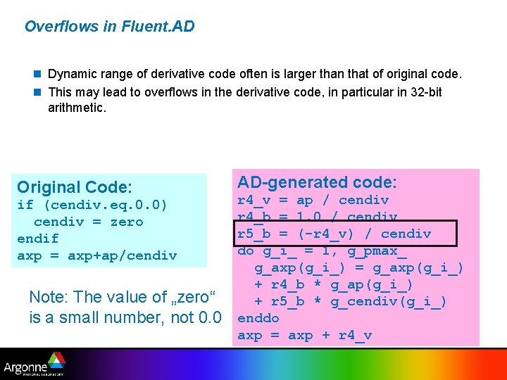
Overflows in Fluent. AD n Dynamic range of derivative code often is larger than that of original code. n This may lead to overflows in the derivative code, in particular in 32 -bit arithmetic. Original Code: if (cendiv. eq. 0. 0) cendiv = zero endif axp = axp+ap/cendiv Note: The value of „zero“ is a small number, not 0. 0 AD-generated code: r 4_v = ap / cendiv r 4_b = 1. 0 / cendiv r 5_b = (-r 4_v) / cendiv do g_i_ = 1, g_pmax_ g_axp(g_i_) = g_axp(g_i_) + r 4_b * g_ap(g_i_) + r 5_b * g_cendiv(g_i_) enddo axp = axp + r 4_v

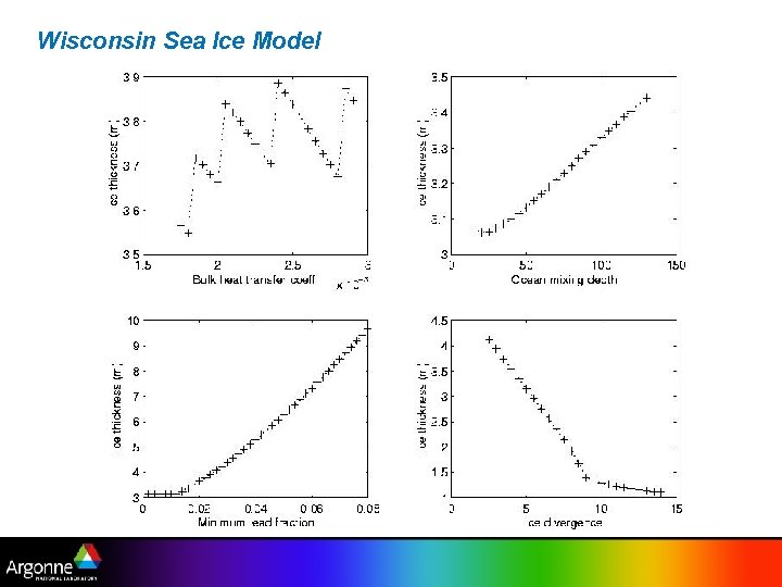
Wisconsin Sea Ice Model

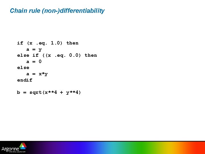
Chain rule (non-)differentiability if (x. eq. 1. 0) then a = y else if ((x. eq. 0. 0) then a = 0 else a = x*y endif b = sqrt(x**4 + y**4)

Mathematical Challenges n Derivatives of intrinsic functions at points of non-differentiability n Derivatives of implicitly defined functions n Derivatives of functions computed using numerical methods

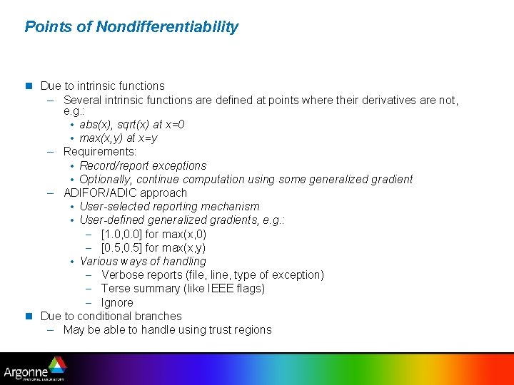
Points of Nondifferentiability n Due to intrinsic functions – Several intrinsic functions are defined at points where their derivatives are not, e. g. : • abs(x), sqrt(x) at x=0 • max(x, y) at x=y – Requirements: • Record/report exceptions • Optionally, continue computation using some generalized gradient – ADIFOR/ADIC approach • User-selected reporting mechanism • User-defined generalized gradients, e. g. : – [1. 0, 0. 0] for max(x, 0) – [0. 5, 0. 5] for max(x, y) • Various ways of handling – Verbose reports (file, line, type of exception) – Terse summary (like IEEE flags) – Ignore n Due to conditional branches – May be able to handle using trust regions

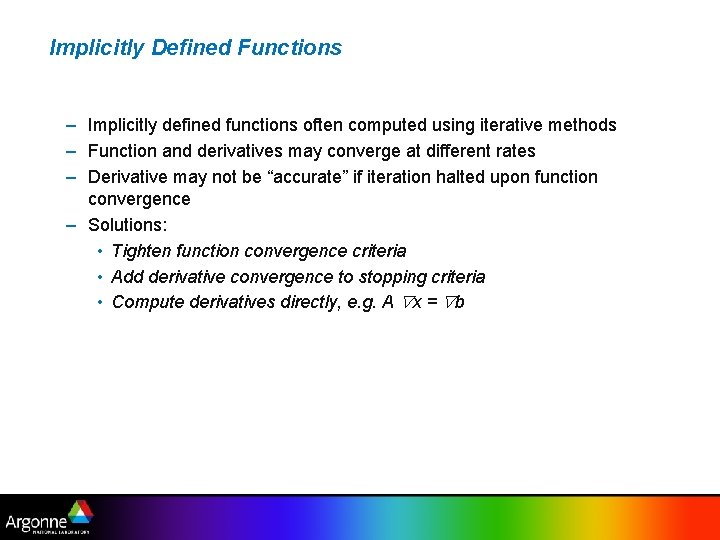
Implicitly Defined Functions – Implicitly defined functions often computed using iterative methods – Function and derivatives may converge at different rates – Derivative may not be “accurate” if iteration halted upon function convergence – Solutions: • Tighten function convergence criteria • Add derivative convergence to stopping criteria • Compute derivatives directly, e. g. A x = b

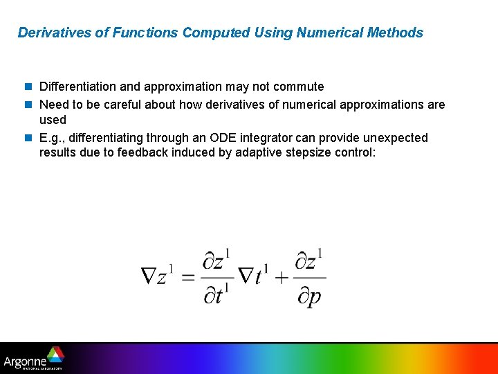
Derivatives of Functions Computed Using Numerical Methods n Differentiation and approximation may not commute n Need to be careful about how derivatives of numerical approximations are used n E. g. , differentiating through an ODE integrator can provide unexpected results due to feedback induced by adaptive stepsize control:

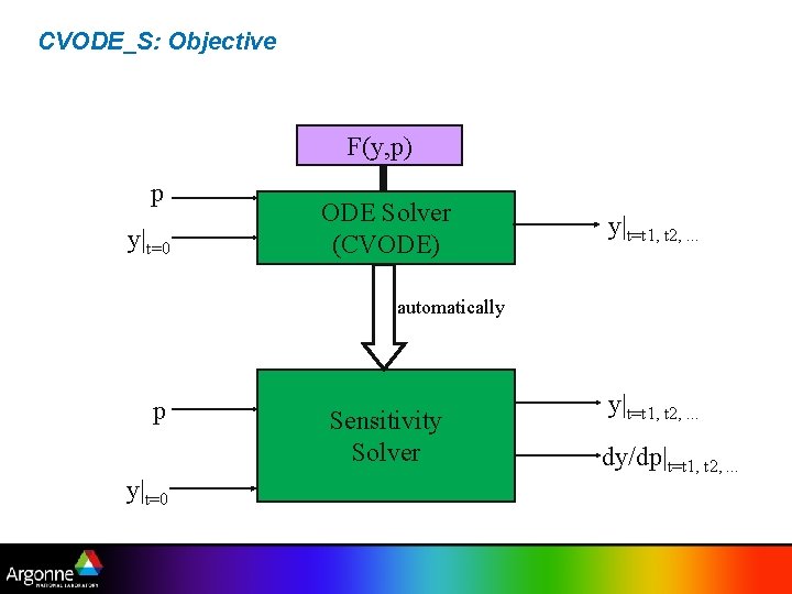
CVODE_S: Objective F(y, p) p y|t=0 ODE Solver (CVODE) y|t=t 1, t 2, . . . automatically p y|t=0 Sensitivity Solver y|t=t 1, t 2, . . . dy/dp|t=t 1, t 2, . . .

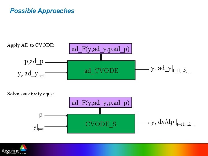
Possible Approaches Apply AD to CVODE: ad_F(y, ad_y, p, ad_p) p, ad_p y, ad_y|t=0 ad_CVODE y, ad_y|t=t 1, t 2, . . . Solve sensitivity eqns: ad_F(y, ad_y, p, ad_p) p y|t=0 CVODE_S y, dy/dp |t=t 1, t 2, . . .

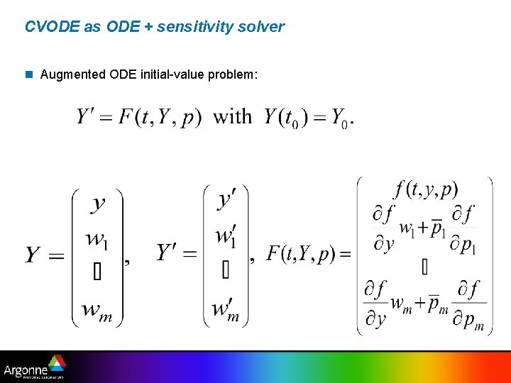
CVODE as ODE + sensitivity solver n Augmented ODE initial-value problem:

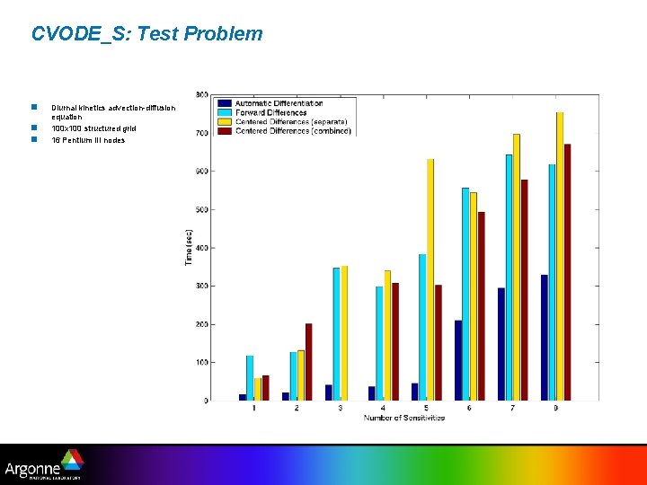
CVODE_S: Test Problem n n n Diurnal kinetics advection-diffusion equation 100 x 100 structured grid 16 Pentium III nodes

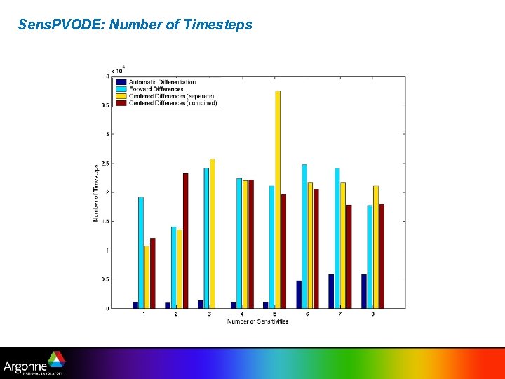
Sens. PVODE: Number of Timesteps

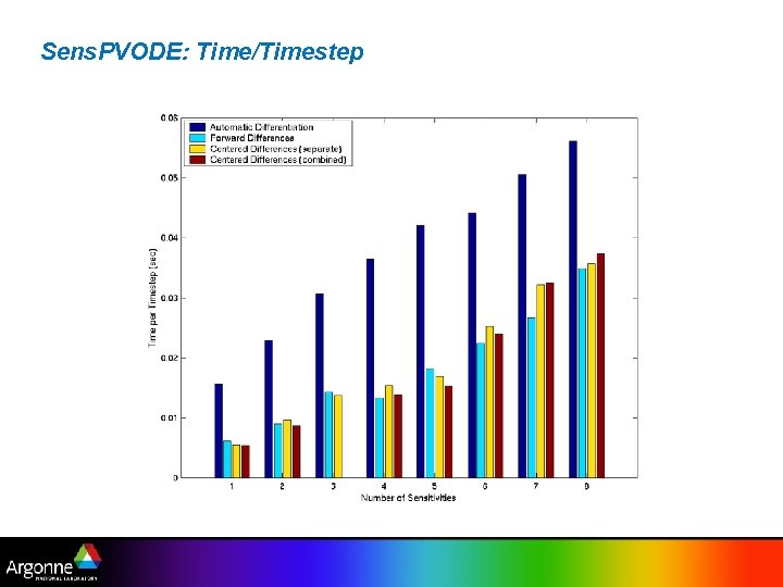
Sens. PVODE: Time/Timestep

Addressing Limitations in Black Box AD n Detect points of nondifferentiability – proceed with a subgradient – currently supported for intrinsic functions, but not conditional statements n Exploit mathematics to avoid differentiating through an adaptive algorithm n Modify termination criterion for implicitly defined functions – Tighten tolerance – Add derivatives to termination test (preferred)

Conclusions n There are some potential “gotchas” when applying AD in a black box fashion n Some care should be taken to ensure that the desired quantity is computed n There are usually workarounds

AD Intro: Follow Up

Practical Matters: constructing computational graphs n At compile time (source transformation) – Structure of graph is known, but edge weights are not: in effect, implement inspector (symbolic) phase at compile time (offline), executor (numeric) phase at run time (online) – In order to assemble graph from individual statements, must be able to resolve aliases, be able to match variable definitions and uses – Scope of computational graph construction is usually limited to statements or basic blocks – Computational graph usually has O(10)—O(100) vertices n At run time (operator overloading) – Structure and weights both discovered at runtime – Completely online—cannot afford polynomial time algorithms to analyze graph – Computational graph may have O(10, 000) vertices

Checkpointing real applications n In practice, need a combination of all of these techniques n At the timestep level, 2 - or 3 -level checkpointing is typical: too many timesteps to checkpoint every timestep n At the call tree level, some mixture of joint and split mode is desirable – Pure split mode consumes too much memory – Pure joint mode wastes time recomputing at the lowest levels of the call tree n Currently, Open. AD provides a templating mechanism to simplify the use of mixed checkpointing strategies n Future research will attempt to automate some of the checkpointing strategy selection, including dynamic adaptation

What to do for very large, dense Jacobian matrices? n Jacobian matrix might be large and dense, but “effectively sparse” – Many entries below some threshold ε (“almost zero”) – Can tolerate errors up to δ in entries greater than ε – Example: advection-diffusion for finite time step: nonlocal terms fall off exponentially – Solution: do a partial coloring to compress this dense Jacobian: requires solving a modified graph coloring problem n Jacobian might be large and dense, but “effectively low rank” – Can be well approximated by a low rank matrix – Jacobian-vector products (and JTv) are cheap – Adaptation of efficient subspace method uses Jv and JTv in random directions to build low rank approximation (Abdel-Khalik et al. , AD 08)

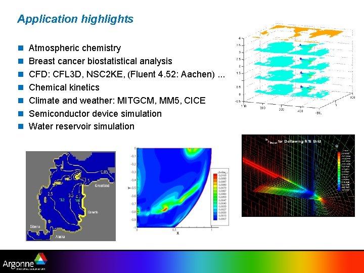
Application highlights n n n n Atmospheric chemistry Breast cancer biostatistical analysis CFD: CFL 3 D, NSC 2 KE, (Fluent 4. 52: Aachen). . . Chemical kinetics Climate and weather: MITGCM, MM 5, CICE Semiconductor device simulation Water reservoir simulation

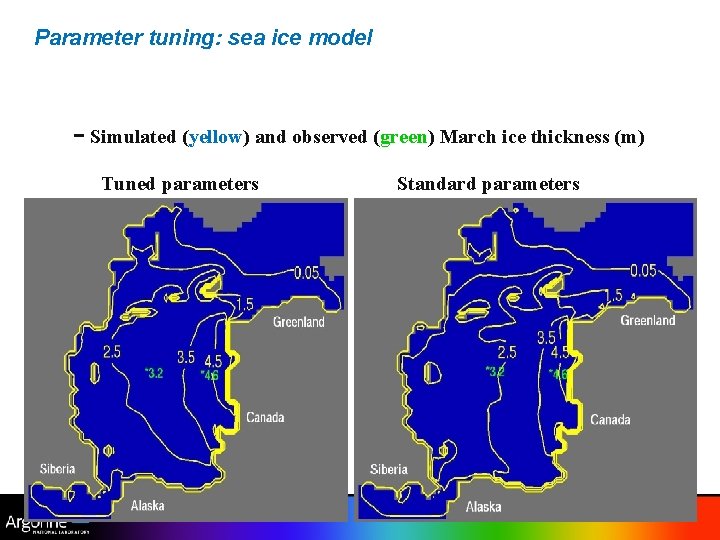
Parameter tuning: sea ice model - Simulated (yellow) and observed (green) March ice thickness (m) Tuned parameters Standard parameters

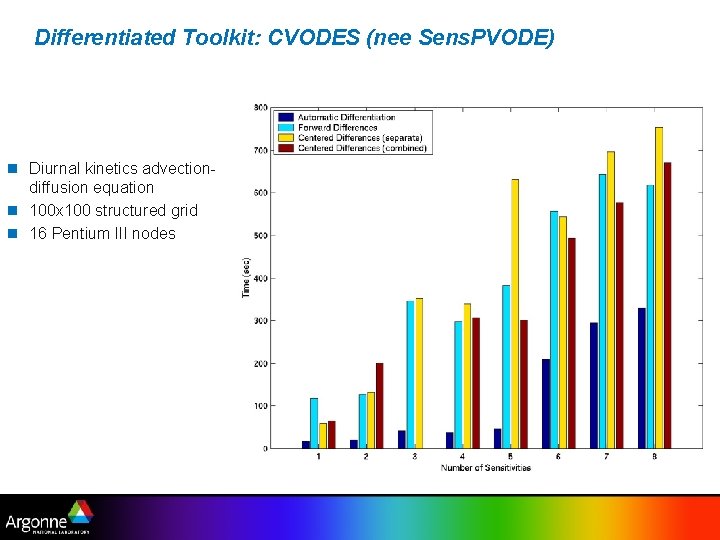
Differentiated Toolkit: CVODES (nee Sens. PVODE) n Diurnal kinetics advectiondiffusion equation n 100 x 100 structured grid n 16 Pentium III nodes

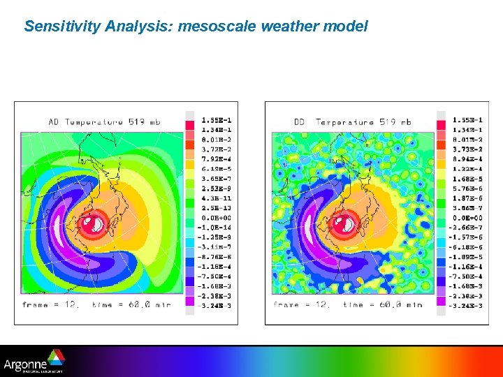
Sensitivity Analysis: mesoscale weather model

Conclusions & Future Work n Automatic differentiation research involves a wide range of combinatorial problems n AD is a powerful tool for scientific computing n Modern automatic differentiation tools are robust and produce efficient code for complex simulation codes – Robustness requires an industrial-strength compiler infrastructure – Efficiency requires sophisticated compiler analysis n Effective use of automatic differentiation depends on insight into problem structure n Future Work – Further develop and test techniques for computing Jacobians that are effectively sparse or effectively low rank – Develop techniques to automatically generate complex and adaptive checkpointing strategies

For More Information n Andreas Griewank, Evaluating Derivatives, SIAM, 2000. n Griewank, “On Automatic Differentiation”; this and other technical reports available online at: http: //www. mcs. anl. gov/autodiff/tech_reports. html n AD in general: http: //www. mcs. anl. gov/autodiff/, http: //www. autodiff. org/ n ADIFOR: http: //www. mcs. anl. gov/adifor/ n ADIC: http: //www. mcs. anl. gov/adic/ n Open. AD: http: //www. mcs. anl. gov/openad/ n Other tools: http: //www. autodiff. org/ n E-mail: hovland@mcs. anl. gov