AUTOMATED MAZE GENERATION AND SOLVING OVER EPOCHS Chad

AUTOMATED MAZE GENERATION AND SOLVING OVER EPOCHS Chad Harris

Informal Definition ■ Rank a collection of three maze generations algorithms according to generation and solve times. ■ Constraints for Measurements – Recording times for generation of mazes strictly tied to core algorithm. – Recording times for solving of mazes strictly tied to universal solve algorithm. ■ Starting and finishing points set at (0, 0) and (n – 1, n – 1) respectively. – Measurements yielded for a maze of n x n size. – Ranking based on ratio of average generation time / average solve time ■ (Closer to zero the better the ranking)

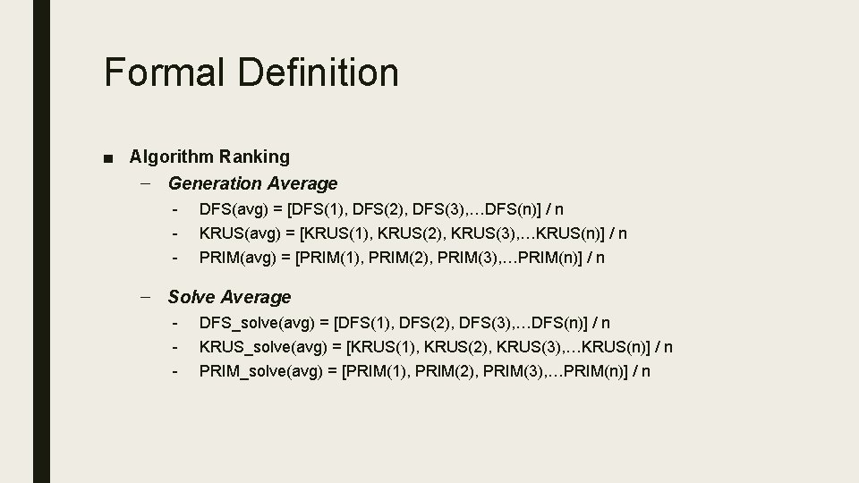
Formal Definition ■ Algorithm Ranking – Generation Average - DFS(avg) = [DFS(1), DFS(2), DFS(3), …DFS(n)] / n KRUS(avg) = [KRUS(1), KRUS(2), KRUS(3), …KRUS(n)] / n PRIM(avg) = [PRIM(1), PRIM(2), PRIM(3), …PRIM(n)] / n – Solve Average - DFS_solve(avg) = [DFS(1), DFS(2), DFS(3), …DFS(n)] / n KRUS_solve(avg) = [KRUS(1), KRUS(2), KRUS(3), …KRUS(n)] / n PRIM_solve(avg) = [PRIM(1), PRIM(2), PRIM(3), …PRIM(n)] / n

Formal Definition (cont’d) – Algorithm Rank - DFS(rank) = [DFS(avg)/DFS_solve(avg)] - KRUS(rank) = [KRUS(avg)/KRUS_solve(avg)] - PRIM(rank) = [PRIM(avg)/PRIM_solve(avg)] – Best Algorithm - ALGO(rank) = {DFS(rank), KRUS(rank), PRIM(rank)} ALGO(rank_optimal)(1) < ALGO(rank)(2) && ALGO(rank_optimal)(1) < ALGO(rank)(3)

Data Representation ■ Adjacency Lists – For cells in all cardinal directions – For open or closed walls for each cell in cardinal directions and cell state

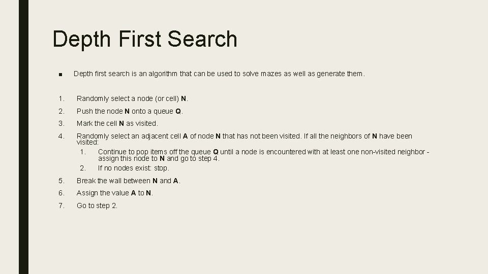
Depth First Search ■ Depth first search is an algorithm that can be used to solve mazes as well as generate them. 1. Randomly select a node (or cell) N. 2. Push the node N onto a queue Q. 3. Mark the cell N as visited. 4. Randomly select an adjacent cell A of node N that has not been visited. If all the neighbors of N have been visited: 1. Continue to pop items off the queue Q until a node is encountered with at least one non-visited neighbor - assign this node to N and go to step 4. 2. If no nodes exist: stop. 5. Break the wall between N and A. 6. Assign the value A to N. 7. Go to step 2.

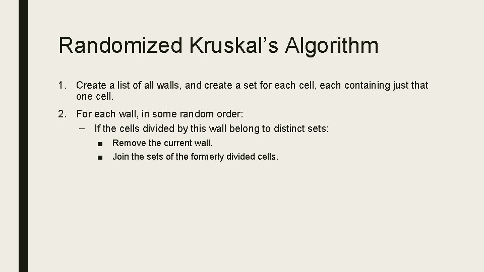
Randomized Kruskal’s Algorithm 1. Create a list of all walls, and create a set for each cell, each containing just that one cell. 2. For each wall, in some random order: – If the cells divided by this wall belong to distinct sets: ■ ■ Remove the current wall. Join the sets of the formerly divided cells.

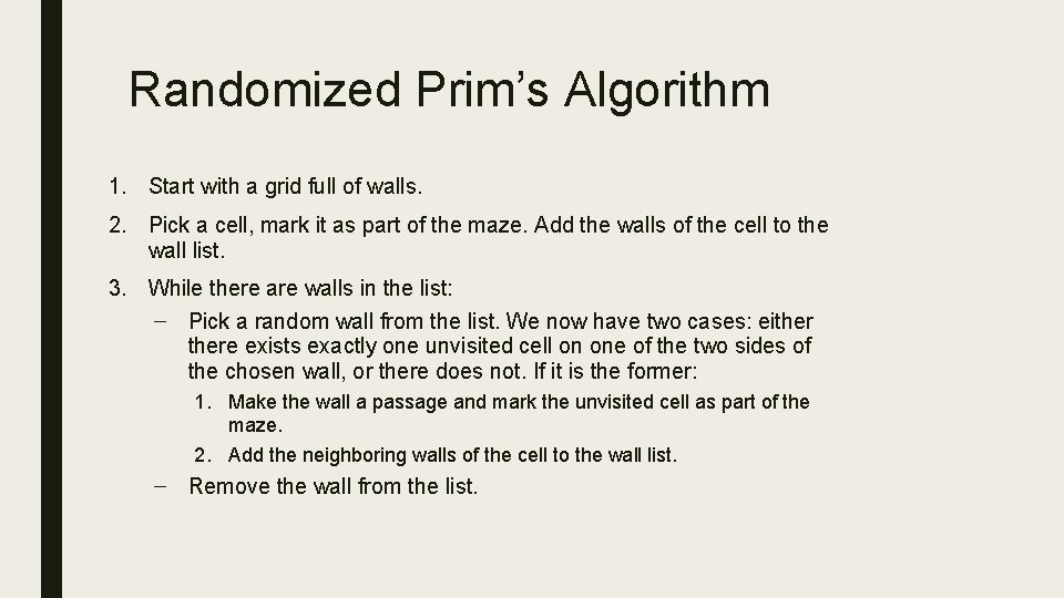
Randomized Prim’s Algorithm 1. Start with a grid full of walls. 2. Pick a cell, mark it as part of the maze. Add the walls of the cell to the wall list. 3. While there are walls in the list: – Pick a random wall from the list. We now have two cases: eithere exists exactly one unvisited cell on one of the two sides of the chosen wall, or there does not. If it is the former: 1. Make the wall a passage and mark the unvisited cell as part of the maze. 2. Add the neighboring walls of the cell to the wall list. – Remove the wall from the list.

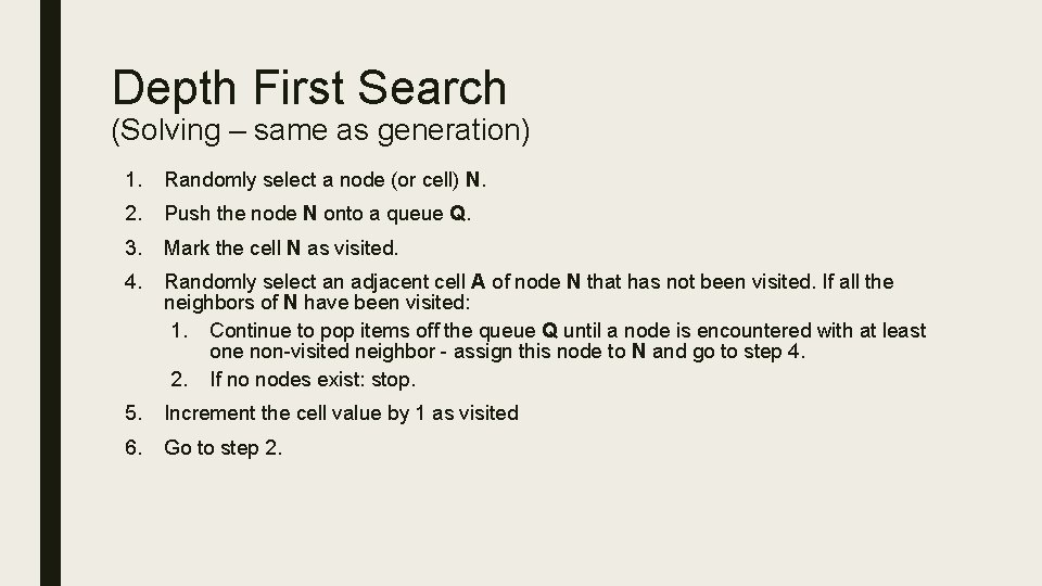
Depth First Search (Solving – same as generation) 1. Randomly select a node (or cell) N. 2. Push the node N onto a queue Q. 3. Mark the cell N as visited. 4. Randomly select an adjacent cell A of node N that has not been visited. If all the neighbors of N have been visited: 1. Continue to pop items off the queue Q until a node is encountered with at least one non-visited neighbor - assign this node to N and go to step 4. 2. If no nodes exist: stop. 5. Increment the cell value by 1 as visited 6. Go to step 2.

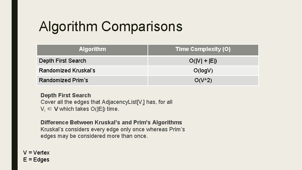
Algorithm Comparisons Algorithm Time Complexity (O) Depth First Search O(|V| + |E|) Randomized Kruskal’s O(log. V) Randomized Prim’s O(V^2) Depth First Search Cover all the edges that Adjacency. List[Vi] has, for all Vi ∈ V which takes O(|E|) time. Difference Between Kruskal’s and Prim’s Algorithms Kruskal’s considers every edge only once whereas Prim’s edges may be considered more than once. V = Vertex E = Edges

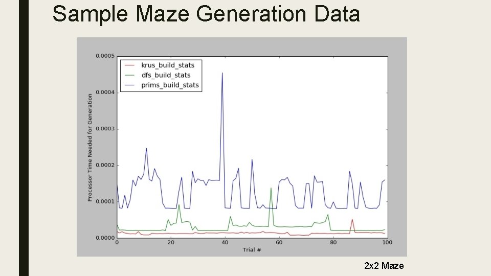
Sample Maze Generation Data 2 x 2 Maze

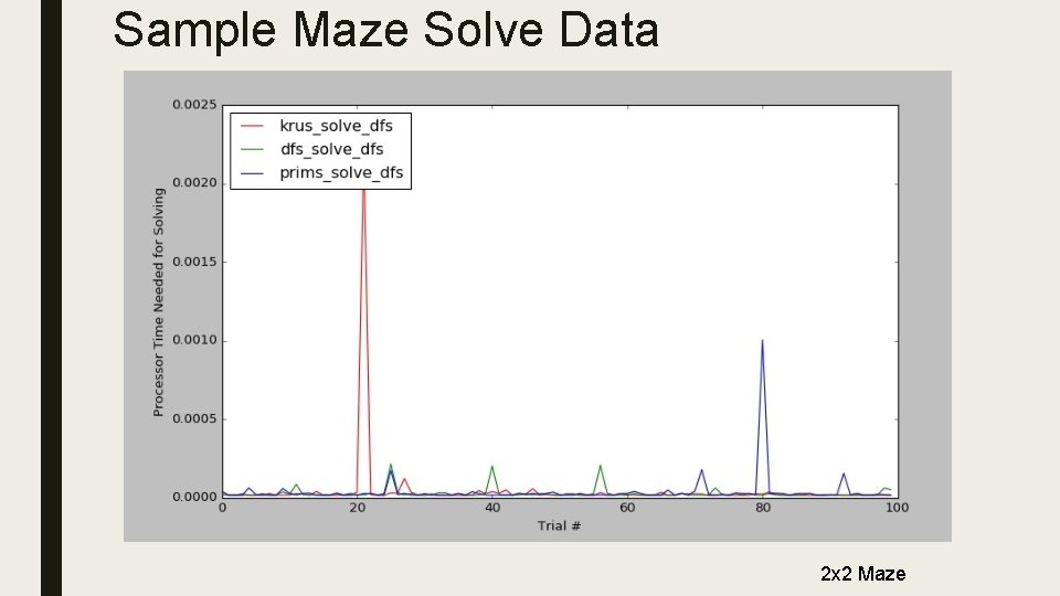
Sample Maze Solve Data 2 x 2 Maze

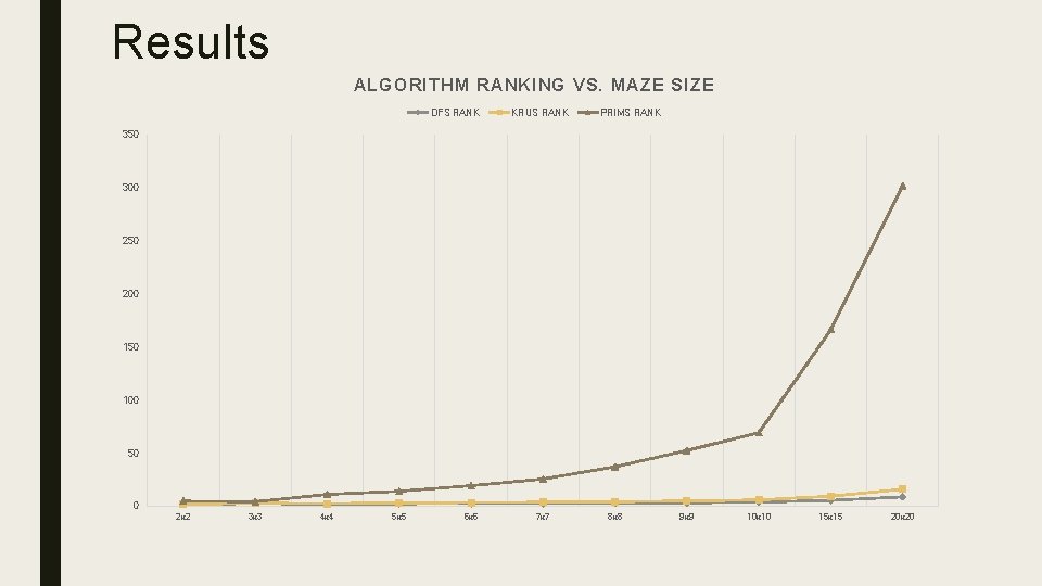
Results ALGORITHM RANKING VS. MAZE SIZE DFS RANK KRUS RANK PRIMS RANK 350 300 250 200 150 100 50 0 2 x 2 3 x 3 4 x 4 5 x 5 6 x 6 7 x 7 8 x 8 9 x 9 10 x 10 15 x 15 20 x 20

Question 1 ■ Q: Which algorithm performed the best over the course of the experiment? ■ A: In all the Kruskal’s algorithm perform the best as the maze size increased. This is due to the runtime efficiency of the algorithm as it is in log(n) time.

Question 2 ■ Q: Why define the start and end points (0, 0) and (n-1, n-1)? ■ A: The purpose in doing this was to allow the complete traversal of the maze for both the creation and solving so that accurate data could be represented as a result of increasing maze size as well as the independent variable in order to accurately compare the efficiency of the algorithms.

Question 3 ■ Q: Which factor contributed the most to the ranking of the algorithms overall? ■ A: The build times associated with each algorithm accounted for the majority of the results. Solve times were harder to disassociate from the data but there are instances where the solve times take longer and improve the ranking of the algorithms in general.

Question 4 ■ Q: What could have been done differently to ensure more accurate results? ■ A: Taking more of an approach to the uniformity of the areas of each algorithm that was recorded and allowing the recording of the processing times to correspond specifically to each step that correlates to each of the other algorithms. (ie. recording procedures that are akin to how the other algorithms were recorded)

Question 5 ■ Q: How would using another or multiple solving algorithms affect the results? ■ A: Using multiple solving algorithms could provide a more accurate measurement for the solving averages however since the greatest factor associated to the ranking of algorithms dealt with the generation times, the averaging of multiple solving algorithms would have little to no benefit to improve overall trends.

QUESTIONS?