Autoencoders Unsupervised Learning and Deep Architectures P Baldi

Autoencoders, Unsupervised Learning, and Deep Architectures P. Baldi University of California, Irvine

1. 2. 3. 4. General Definition Historical Motivation (50 s, 80 s, 2010 s) Linear Autoencoders over Infinite Fields Non-Linear Autoencoders: the Boolean Case 5. Summary and Speculations

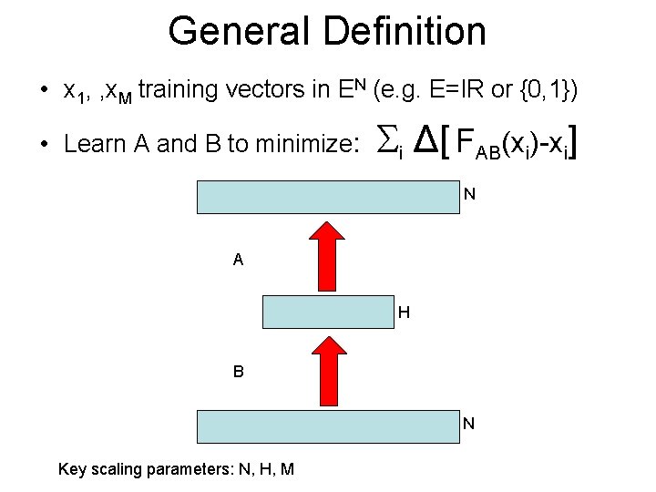
General Definition • x 1, , x. M training vectors in EN (e. g. E=IR or {0, 1}) • Learn A and B to minimize: i Δ[ FAB(xi)-xi] N A H B N Key scaling parameters: N, H, M

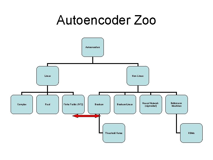
Autoencoder Zoo Autoencoders Linear Complex Real Non-Linear Finite Fields (GF 2) Boolean/Linear Threshold Gates Neural Network (sigmoidal) Boltzmann Machines RBMs

Historical Motivation • Three time periods: 1950 s, 1980 s, 2010 s. • Three motivations: – Fundamental Learning Problem (1950 s) – Unsupervised Learning (1980 s) – Deep Architectures (2010 s)

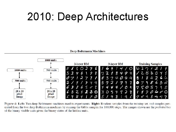
2010: Deep Architectures

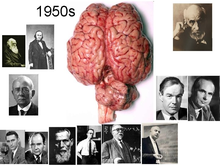
1950 s

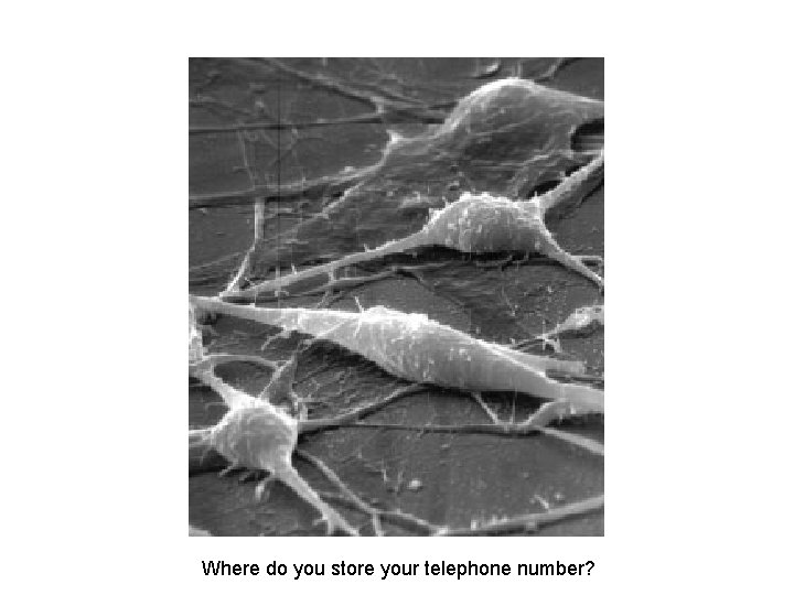
Where do you store your telephone number?

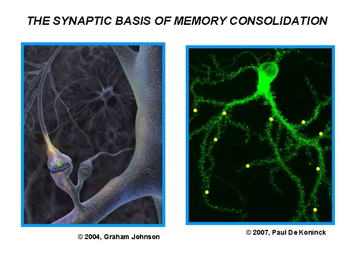
THE SYNAPTIC BASIS OF MEMORY CONSOLIDATION © 2004, Graham Johnson © 2007, Paul De

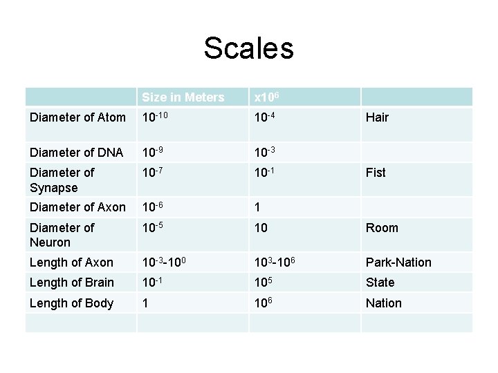
Scales Size in Meters x 106 Diameter of Atom 10 -10 10 -4 Diameter of DNA 10 -9 10 -3 Diameter of Synapse 10 -7 10 -1 Diameter of Axon 10 -6 1 Diameter of Neuron 10 -5 10 Room Length of Axon 10 -3 -100 103 -106 Park-Nation Length of Brain 10 -1 105 State Length of Body 1 106 Nation Hair Fist

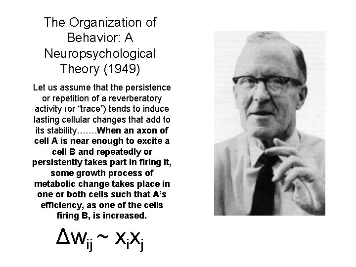
The Organization of Behavior: A Neuropsychological Theory (1949) Let us assume that the persistence or repetition of a reverberatory activity (or “trace”) tends to induce lasting cellular changes that add to its stability……. When an axon of cell A is near enough to excite a cell B and repeatedly or persistently takes part in firing it, some growth process of metabolic change takes place in one or both cells such that A’s efficiency, as one of the cells firing B, is increased. Δwij ~ xixj

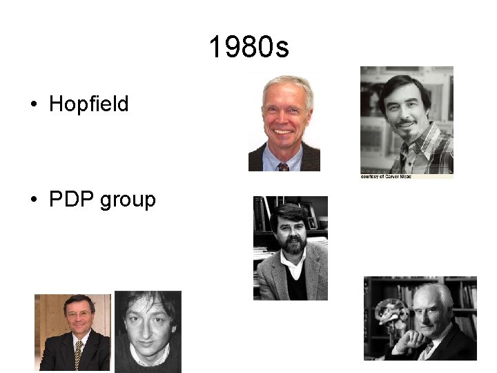
1980 s • Hopfield • PDP group

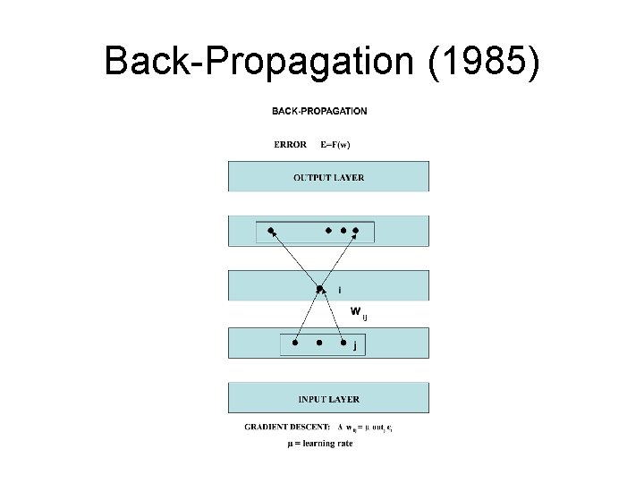
Back-Propagation (1985)

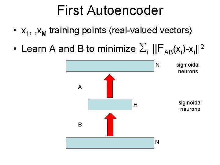
First Autoencoder • x 1, , x. M training points (real-valued vectors) • Learn A and B to minimize i ||FAB(xi)-xi||2 N sigmoidal neurons A sigmoidal neurons H B N

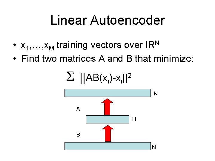
Linear Autoencoder • x 1, …, x. M training vectors over IRN • Find two matrices A and B that minimize: i ||AB(xi)-xi||2 N A H B N

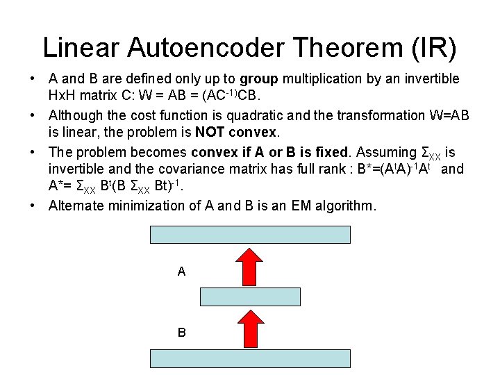
Linear Autoencoder Theorem (IR) • A and B are defined only up to group multiplication by an invertible Hx. H matrix C: W = AB = (AC-1)CB. • Although the cost function is quadratic and the transformation W=AB is linear, the problem is NOT convex. • The problem becomes convex if A or B is fixed. Assuming ΣXX is invertible and the covariance matrix has full rank : B*=(At. A)-1 At and A*= ΣXX Bt(B ΣXX Bt)-1. • Alternate minimization of A and B is an EM algorithm. A B

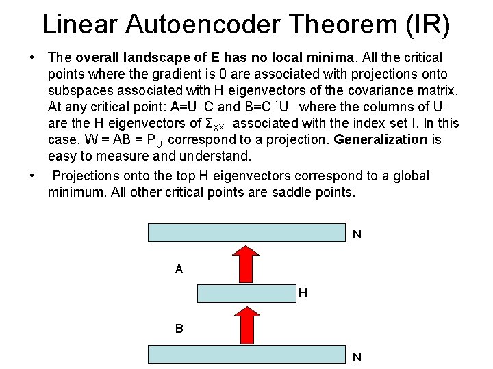
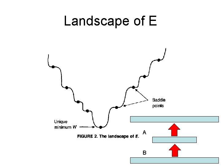
Linear Autoencoder Theorem (IR) • The overall landscape of E has no local minima. All the critical points where the gradient is 0 are associated with projections onto subspaces associated with H eigenvectors of the covariance matrix. At any critical point: A=UI C and B=C-1 UI where the columns of UI are the H eigenvectors of ΣXX associated with the index set I. In this case, W = AB = PUI correspond to a projection. Generalization is easy to measure and understand. • Projections onto the top H eigenvectors correspond to a global minimum. All other critical points are saddle points. N A H B N

Landscape of E A B

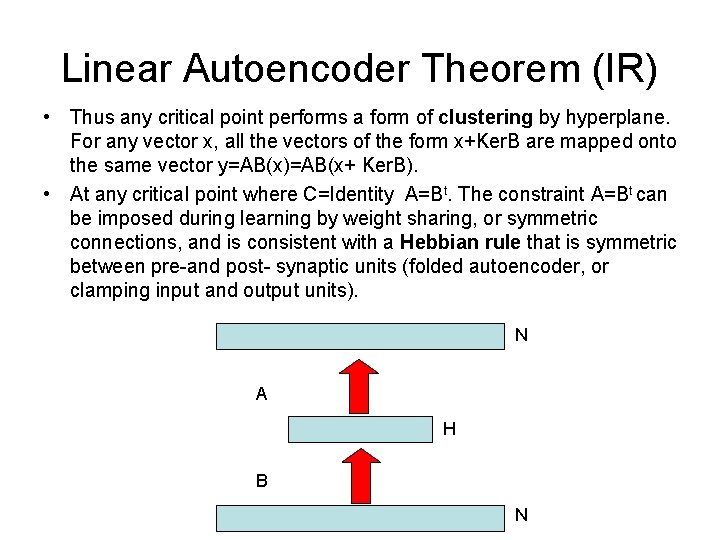
Linear Autoencoder Theorem (IR) • Thus any critical point performs a form of clustering by hyperplane. For any vector x, all the vectors of the form x+Ker. B are mapped onto the same vector y=AB(x)=AB(x+ Ker. B). • At any critical point where C=Identity A=Bt. The constraint A=Bt can be imposed during learning by weight sharing, or symmetric connections, and is consistent with a Hebbian rule that is symmetric between pre-and post- synaptic units (folded autoencoder, or clamping input and output units). N A H B N

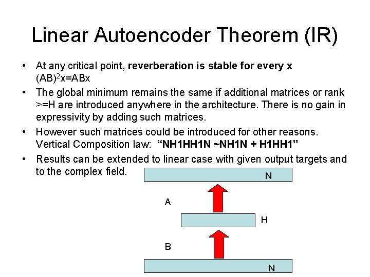
Linear Autoencoder Theorem (IR) • At any critical point, reverberation is stable for every x (AB)2 x=ABx • The global minimum remains the same if additional matrices or rank >=H are introduced anywhere in the architecture. There is no gain in expressivity by adding such matrices. • However such matrices could be introduced for other reasons. Vertical Composition law: “NH 1 HH 1 N ~NH 1 N + H 1 HH 1” • Results can be extended to linear case with given output targets and to the complex field. N A H B N

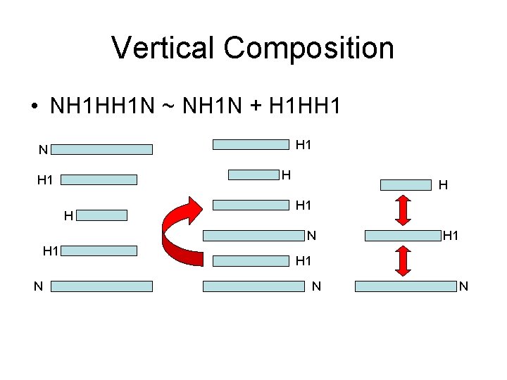
Vertical Composition • NH 1 HH 1 N ~ NH 1 N + H 1 HH 1 N H H 1 H H H 1 N N

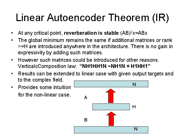
Linear Autoencoder Theorem (IR) • At any critical point, reverberation is stable (AB)2 x=ABx • The global minimum remains the same if additional matrices or rank >=H are introduced anywhere in the architecture. There is no gain in expressivity by adding such matrices. • However such matrices could be introduced for other reasons. Verticalc. Composition law: “NH 1 HH 1 N ~NH 1 N + H 1 HH 1” • Results can be extended to linear case with given output targets and to the complex field. N • Provides some intuition for the non-linear case. A H B N

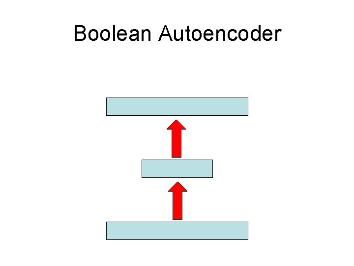
Boolean Autoencoder

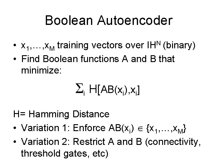
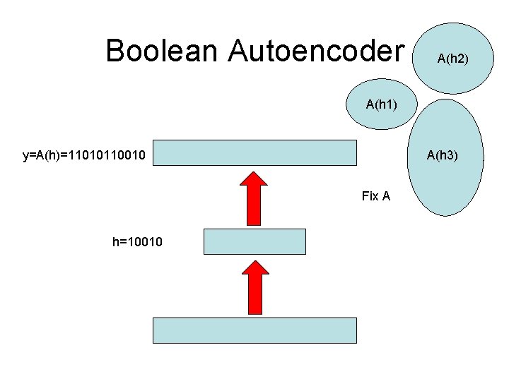
Boolean Autoencoder • x 1, …, x. M training vectors over IHN (binary) • Find Boolean functions A and B that minimize: i H[AB(xi), xi] H= Hamming Distance • Variation 1: Enforce AB(xi) {x 1, …, x. M} • Variation 2: Restrict A and B (connectivity, threshold gates, etc)

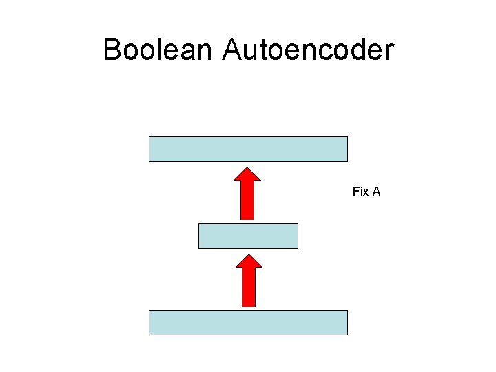
Boolean Autoencoder Fix A

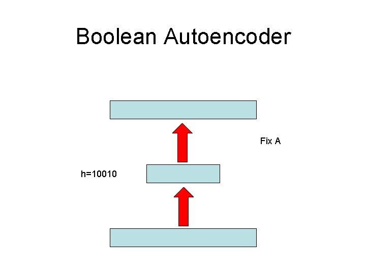
Boolean Autoencoder Fix A h=10010

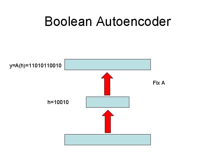
Boolean Autoencoder y=A(h)=11010110010 Fix A h=10010

Boolean Autoencoder A(h 2) A(h 1) y=A(h)=11010110010 A(h 3) Fix A h=10010

Autoencoder A(h 2) A(h 1) y=A(h)=11010110010 A(h 3) Fix A h=10010 B({Voronoi A(h)}) =h

Boolean Autoencoder Fix B

Boolean Autoencoder A h=10100 Fix B

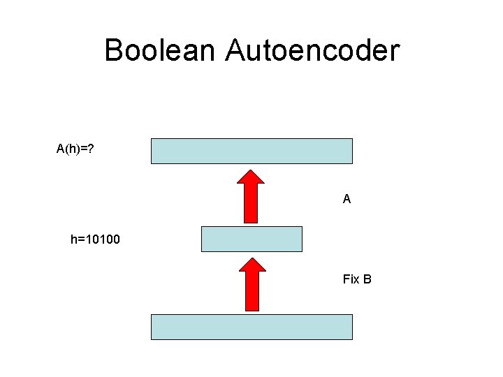
Boolean Autoencoder A(h)=? A h=10100 Fix B

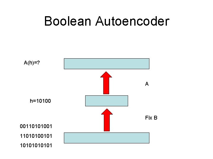
Boolean Autoencoder A(h)=? A h=10100 Fix B 0011010100101 1010101

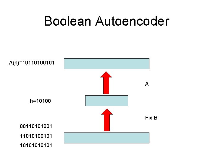
Boolean Autoencoder A(h)=10110100101 A h=10100 Fix B 0011010100101 1010101

Boolean Autoencoder A(h)=Majority[B-1(h)] A(h)=10110100101 A h=10100 Fix B 0011010100101 1010101

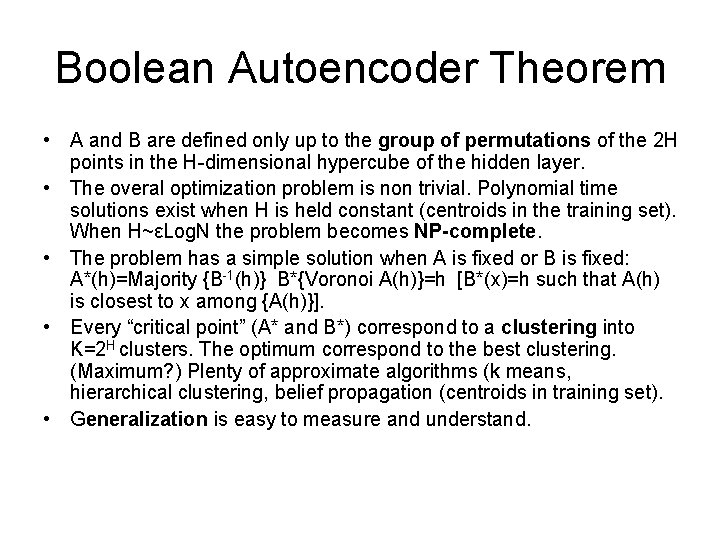
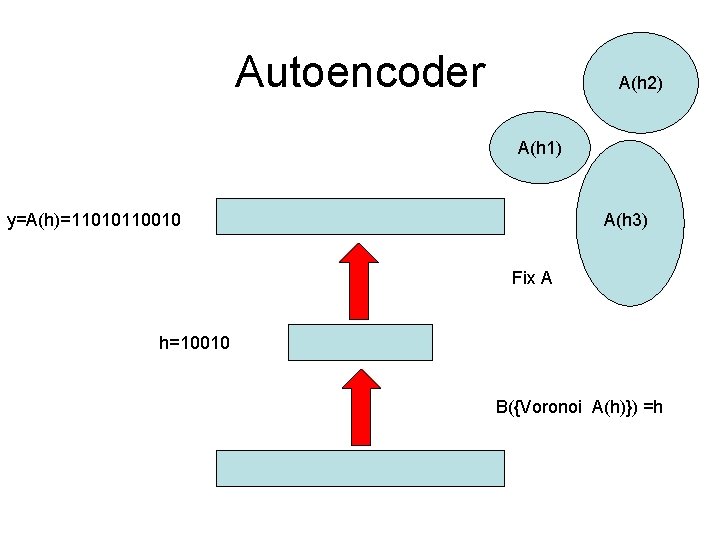
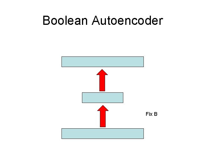
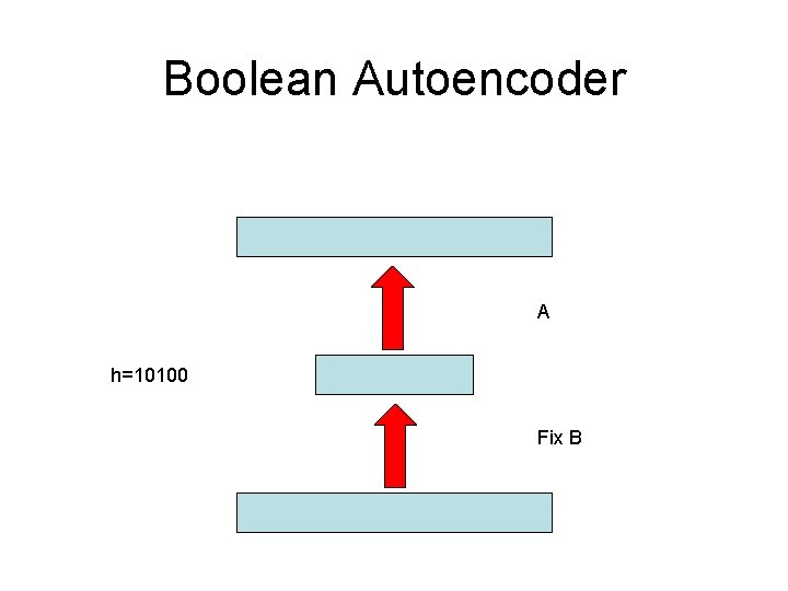
Boolean Autoencoder Theorem • A and B are defined only up to the group of permutations of the 2 H points in the H-dimensional hypercube of the hidden layer. • The overal optimization problem is non trivial. Polynomial time solutions exist when H is held constant (centroids in the training set). When H~εLog. N the problem becomes NP-complete. • The problem has a simple solution when A is fixed or B is fixed: A*(h)=Majority {B-1(h)} B*{Voronoi A(h)}=h [B*(x)=h such that A(h) is closest to x among {A(h)}]. • Every “critical point” (A* and B*) correspond to a clustering into K=2 H clusters. The optimum correspond to the best clustering. (Maximum? ) Plenty of approximate algorithms (k means, hierarchical clustering, belief propagation (centroids in training set). • Generalization is easy to measure and understand.

Boolean Autoencoder Theorem • At any critical point, reverberation is stable. • The global minimum remains the same if additional Boolean functions with layers >=H are introduced anywhere in the architecture. There is no gain in expressivity by adding such functions. • However such functions could be introduced for other reasons. Composition law: “NH 1 HH 1 N ~NH 1 N + H 1 HH 1”. Can achieve hierarchical clustering in input space. • Results can be extended to the case with given output targets.

Learning Complexity • Linear autoencoder over infinite fields can be solved analytically • Boolean autoencoder is NP complete as soon as the number of clusters (K=2 H) scales like Mε (for ε>0). It is solvable in polynomial time when K is fixed. • Linear autoencoder over finite fields is NP complete in the general case. • RBM learning is NP complete in the general case.

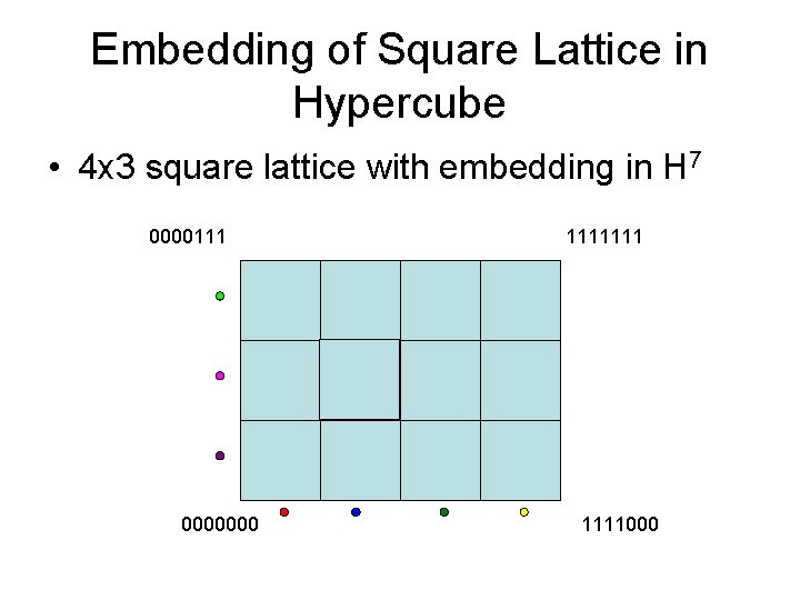
Embedding of Square Lattice in Hypercube • 4 x 3 square lattice with embedding in H 7 0000111 0000000 1111111000

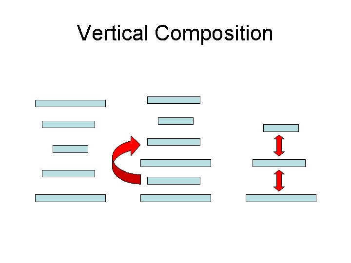
Vertical Composition

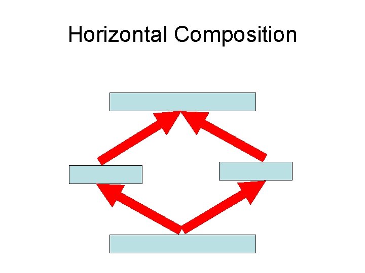
Horizontal Composition

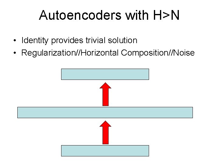
Autoencoders with H>N • Identity provides trivial solution • Regularization//Horizontal Composition//Noise

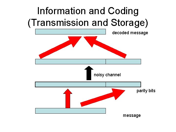
Information and Coding (Transmission and Storage) decoded message noisy channel parity bits message

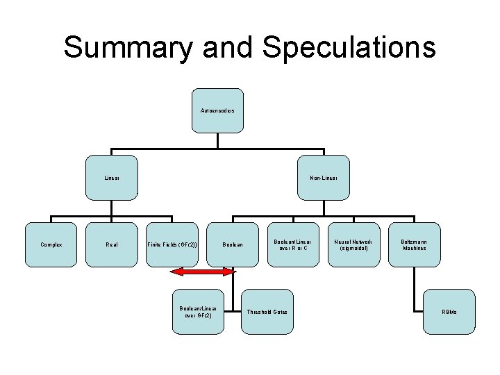
Summary and Speculations Autoencoders Linear Complex Real Non-Linear Finite Fields (GF(2)) Boolean/Linear over GF(2) Boolean/Linear over R or C Threshold Gates Neural Network (sigmoidal) Boltzmann Machines RBMs

Unsupervised Learning Clustering Autoencoders Hebbian Learning

Information and Coding Theory Compression Autoencoders Communication

Deep Architectures Vertical Composition Autoencoders Horizontal Composition

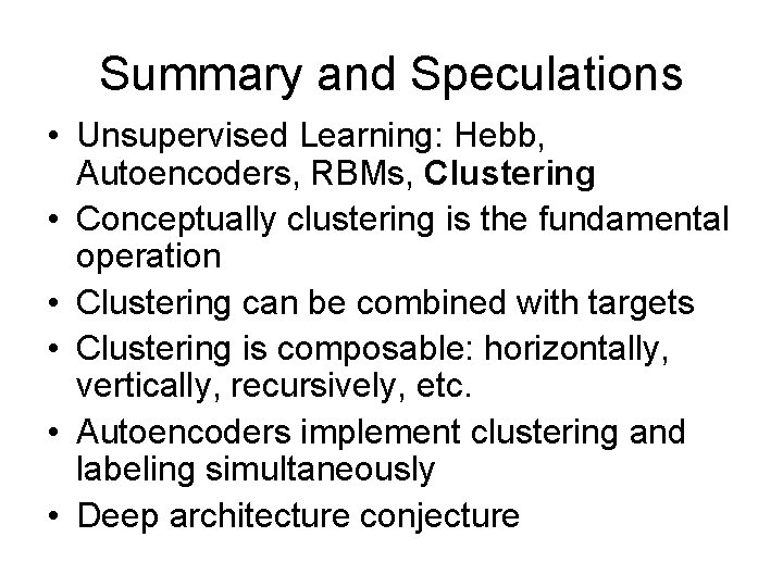
Summary and Speculations • Unsupervised Learning: Hebb, Autoencoders, RBMs, Clustering • Conceptually clustering is the fundamental operation • Clustering can be combined with targets • Clustering is composable: horizontally, vertically, recursively, etc. • Autoencoders implement clustering and labeling simultaneously • Deep architecture conjecture