Autoencoders David Dohan Unsupervised Deep Learning So far

Autoencoders David Dohan

Unsupervised Deep Learning • So far: supervised models • Multilayer perceptrons (MLP) • Convolutional NN (CNN) • Up next: unsupervised models • Autoencoders (AE) • Deep Boltzmann Machines (DBM)

The Goal • Build high-level representations from large unlabeled datasets • Feature learning • Dimensionality reduction • A good representation may be: • Compressed • Sparse • Robust

Hierarchical Representation

The Goal • Uncover implicit structure in unlabeled data • Use labelled data to finetune the learned representation • Better initialization for traditional backpropagation • Semi-supervised learning

Manifold Hypothesis • Realistic data clusters along a manifold • Natural images v. static • Discovering a manifold, assigning coordinate system to it

Manifold Hypothesis • Realistic data clusters along a manifold • Natural images v. static • Discovering a manifold, assigning coordinate system to it

Principal Component Analysis Reduce dimensions by keeping directions of most variance Direction of first principal component i. e. direction of greatest variance

Principal Component Analysis Given N x d data matrix X, want to project using largest m components 1. Zero mean columns of X 2. Calculate SVD of X = UΣV 3. Take W to be first m columns of V 4. Project data by Y = XW Output Y is N x m matrix

Autoencoder Structure • Input, hidden, output layers • Learning encoder to and decoder from feature space • Information bottleneck

Shallow Autoencoder • AE with 2 hidden layers • Try to make the output be the same as the input in a network with a central bottleneck. output vector code input vector • The activities of the hidden units in the bottleneck form an efficient code. • Similar to PCA if layers are linear

Shallow Autoencoder

Shallow Autoencoder

Deep Autoencoder • Non-linear layers allow an AE to represent data on a non-linear manifold • Can initialize MLP by replacing decoding layers with a softmax classifier output vector Decoding weights code Encoding weights input vector

Training Autoencoders • Backpropagation • Trained to approximate the identity function • Minimize reconstruction error • Objectives: • Mean Squared Error: • Cross Entropy:

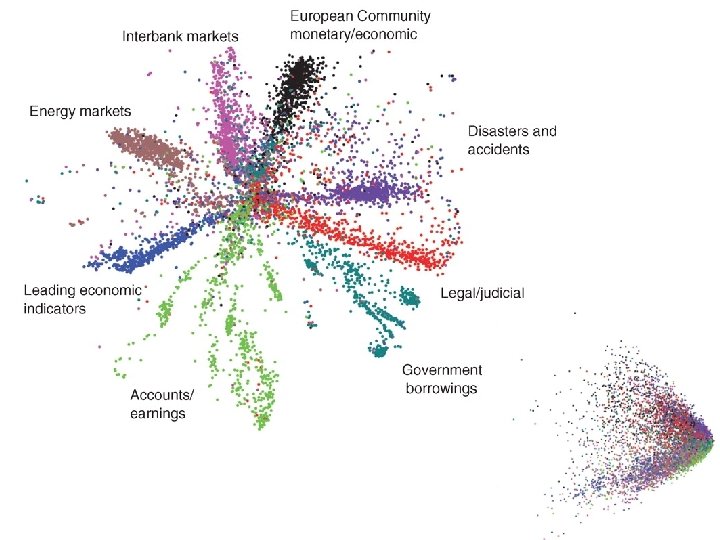
Reconstruction Example Data 30 -D AE 30 -D PCA

Learned Filters • Each image represents a neuron • Color represents connection strength to that pixel • Trained on MNIST dataset

Learned Filters • Trained on natural image patches • Get Gabor-filter like receptive fields

Deep Autoencoder • Face “vanishing gradient” problem • Solution: Greedy layer-wise pretraining • First approach used RBMs (Up next!) • Can initialize with several shallow AE 100 W 4 50 100 W 4 W 3 10 50 W 1 100 50 10 W 2 50 W 1 100

Denoising Autoencoder • Want to prevent AE from learning identity function • Corrupt input during training • Still train to reconstruct input • Forces learning correlations in data • Leads to higher quality features • Capable of learning overcomplete codes

Denoising Autoencoder Web Demo

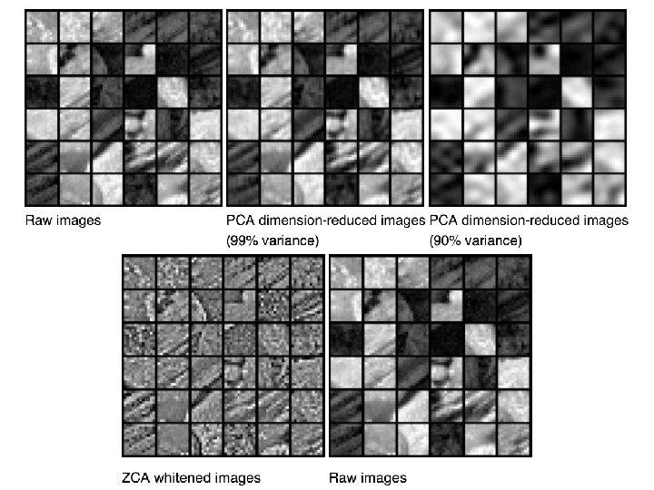
Whitening • AE work best for data with all features equal variance • PCA whitening – Rotate data to principal axes – Take top K eigenvectors – Rescale each feature to have unit variance Implementation Details

Additional Resources • Unsupervised Feature Learning and Deep Learning Tutorial • http: //ufldl. stanford. edu/wiki/ • deeplearning. net/tutorial/ • Thorough introduction to main topics in deep learning

Deep Boltzmann Machines David Dohan

Generative Models • Discriminative models learn p(y | x) • Probability of a label given some input • Generative models instead model p(x) • Sample model to generate new values

Boltzmann Machines (BM) • • • Visible and hidden layers Stochastic binary units Fully connected Undirected Difficult to train

Energy of a Joint Configuration Visible-Hidden connections Visible-Visible connections Hidden-Hidden connections • vi, hi are binary states • Notice that the energy of any connection is local • Only depends on connection strength and state of endpoints Visible Bias Hidden Bias

Energy Based Models • Assign an energy to possible configurations • For no connections, map to probability with: • v is a vector representing a configuration • Denominator is normalizing constant Z • Intractable in real systems • Requires summing over 2 n states • Low energy → high probability

Energy Based Models • Use hidden units to model more abstract relationships between visible units • With hidden units and connections: • θ is model parameters (e. g. connection weight) • v, h vectors representing a layer configuration • Similar form to Boltzmann distribution, therefore Boltzmann machines

Energy Based Models • This is equivalent to defining the probability of a configuration to be the probability of finding the network in that configuration after many stochastic updates

Hidden Variables • Latent factors/explanations for data • Example: movie prediction +1

Restricted BM (RBM) • Remove visible-visible and hidden-hidden connections • Hidden units conditionally independent given visible units (and vice-versa) • Makes training tractable +1

Energy of an RBM • For n visible and m hidden units • W is n x m weight matrix • θ denotes parameters W, b, c • b, v length n row vectors • c, h length m row vectors • Equation represents: (vis↔hid) + visible bias + hidden bias

Inference in RBMs • Conditional distribution of visible and hidden units given by • Each layer distribution completely determined given other layer • Given v, is exact

RBM Training • Maximizing likelihood of training examples v using SGD • First term is exact • Calculate for every example • Second term must be approximated

RBM Training • Consider the gradient of a single example v • First term is exactly • Approximate second term by taking many samples from model and averaging across them

RBM Training • Bias terms are even simpler • Treat as a unit that is always on

Sampling in an RBM • Approximate model expectation by drawing many samples and averaging • Stochastically update each unit based on input • Initialize randomly

Sampling in an RBM • Update each layer in parallel • Alternate layers • Known as a markov chain or fantasy particle

Contrastive Divergence (CD) • Reaching convergence while sampling may take hundreds of steps • K step contrastive divergence (CD-k) • Use only k sampling steps to approximate the expectations • Initialize chains to training example • Much less computationally expensive • Found to work well in practice

RBM Pseudocode Notice that hpos is real valued while vneg is binary

RBM Pseudocode

Persistent CD (PCD) • Markov chains persist between updates • Allows chains to explore energy landscape • Much better generative models in practice

Persistent CD (PCD) • In CD, # chains = batch size • Initialized to data in the batch • Any # of chains in PCD • Initialized once, allowed to run • More chains lead to more accurate expectation

KL Divergence • Measure of difference between probability distributions • CD learning minimizes KL divergence between data and model distributions • NOT the log likelihood

Deep Belief Networks (DBNs) • Limitations on what a single layer model can efficiently represent • Want to learn multi-layer models • Create a stack of easy to train RBMs

Greedy Layer-wise Pretraining Greedy layer-by-layer learning: • Learn and freeze W 1 • Sample h 1 ~ P(h | v, W 1) treat h 1 as if it were data • Learn and freeze W 2 • … • Repeat

Greedy Layer-wise Pretraining • Each extra layer improves lower bound on log probability of data • Additional layers capture higher-order correlations between unit activities in the layer below

Deep Belief Networks (DBNs) • Top two layers from an RBM • Other connections directed • Can generate a sample by sampling back and forth in top two layers before propagating down to visible layers

Greedy Layer-wise Pretraining Web Demo

Deep Boltzmann Machines • All connections undirected • Bottom-up and top-down input to each layer • Use layer-wise pretraining followed by joint training of all layers

Pretraining DBMs • Layerwise pretraining • Must account for input doubling for each layer

Joint Training of DBMs • Pretraining initializes parameters to favorable settings for joint training • Update equations take same basic form: • Model statistic remains intractable • Approximate with PCD • Data statistic, which was exact in the RBM, must also be approximated

Data Dependent Statistic • No longer exact in DBM • Approximate with mean-field variational inference • Clamp data, sample back and forth in hidden layers • Use expectation instead of binary state

Model Dependent Statistic • Approximate with gibbs sampling as in an RBM • Always use PCD • Alternate sampling even/odd layers

Finetuning for Classification • Can use to initialize MLP for classification • Ideal with lots of unsupervised and little supervised data

Semi-supervised Learning • Makes use of unlabelled data together with some labelled data • Initialize by training a generative model of the data • Slightly adjust for discriminative tasks using the labelled data • Most of the parameters come from generative model

Sparsity • Hidden units that are rarely active may be easier to interpret or better for discriminative tasks • Add a “sparsity penalty” to the objective • Target sparsity: want each unit on in a fraction p of the training data • Actual sparsity • Used to adjust bias and weights for each hidden unit

Initializing Autoencoders

Example: Shape. BM • Weight sharing and sparse connections • Each layer models a different part of the data

Example: Shape. BM • Used DBM-like structure to learn a shape prior for segmentation • Good showcase of generative completion abilities

Completing unknown data • Repeatedly sample from model • For any visible layer sample, clamp known locations to the known values

Extensions • Gaussian RBM for image data • Convolutional RBM

Accelerating Training • Most operations are implemented as large matrix multiplications • Use optimized BLAS libraries • Matlab, Open. BLAS, Intel. MKL • GPUs can accelerate most operations • CUDA • Matlab Parallel Computing Toolbox • Theano

RBM Example Code Example Matlab code

Additional Resources • http: //goo. gl/UWt. RWT • Neural Networks, deep learning, and sparse coding course videos from Hugo Larochelle • A Practical Guide to Training RBMs • http: //www. cs. toronto. edu/~hinton/ absps/guide. TR. pdf