Autocorrelation Dr S Selva Arul Pandian Assistant Professor

Autocorrelation Dr. S. Selva Arul Pandian Assistant Professor Department of Statistics Loyola College

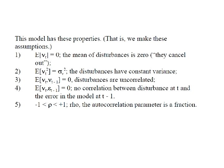
Fundamental assumptions in MLRM about error term

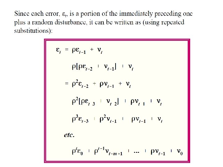
Autocorrelation In some applications of Regression model • The response and regressor variable arranged in sequential order over time (Time Series Data) • Auto correlation is a characteristic of data which shows the degree of similarity between the values of the same variables over successive time intervals. • The existence of autocorrelation in the residuals of a model is a sign that the model may be unsound. • The auto part of autocorrelation is from the Greek word for self, and autocorrelation means data that is correlated with itself

Autocorrelation For example v The column to the right shows the last eight of these values, moved “up” one row, with the first value deleted. v When we correlate these two columns of data, excluding the last observation that has missing values, the correlation is 0. 64. v This means that the data is correlated with itself (i. e. , we have autocorrelation/serial correlation).

Positive and negative autocorrelation • The example above shows positive first-order autocorrelation, where first order indicates that observations that are one apart are correlated, and positive means that the correlation between the observations is positive. • When data exhibiting positive first-order correlation is plotted, the points appear in a smooth snake-like curve, as on the left. With negative first-order correlation, the points form a zigzag pattern if connected, as shown on the right.

Diagnosing autocorrelation using a correlogram • A correlogram shows the correlation of a series of data with itself; it is also known as an autocorrelation plot and an ACF plot. • The lag refers to the order of correlation. We can see in this plot that at lag 0, the correlation is 1, as the data is correlated with itself. • At a lag of 1, the correlation is shown as being around 0. 5 (this is different to the correlation computed above, as the correlogram uses a slightly different formula). • We can also see that we have negative correlations when the points are 3, 4, and 5 apart.

Correlogram

Autocorrelation effects on OLS in Regression • The estimated parameters is still unbiased but variance is not minimum, the estimates are inefficient. • If the errors are positively correlated, error mean square may underestimate the variance and consequently SE of regression coefficient is to small • CI are shorter than they really should be • Testing procedure indicates that one or more regressors contribute significantly to the model but reality does not • CI and Testing of hypothesis are not appropriate (t and F)

Autocorrelation

Another view of Autocorrelation

Why does Autocorrelation occur • When an important regressor variable is not included in the model • When we specify incorrect functional form • Data manipulation • Data transformation

Non Stationarity: Mean, Variance and covariance are time invariant

Detecting Autocorrelation • • Graphical method Run Test Durbin – Watson Test Breush – Godfry (BG Test)

Graphical Method • Find the error terms from OLS estimation. Plot these residuals against time • Positive Correlation

Graphical Method Negative Correlation

Run Test

Run Test