Auditory Perception from Neuron to Cognition and Behaviour

Auditory Perception: from Neuron to Cognition and Behaviour John van Opstal Institute for Neuroscience Dept. of Biophysics Radboud University Nijmegen

Detailed section through the cochlea: Outer Hair cells Organ of Corti Inner Hair cell Auditory nerve Basilar Membrane

Tonotopic organization of the Cochlea: Originates from: • Instantaneous coupling of the BM to the intra-cochlear fluid • Location-dependent stiffness of the BM (Von Békésy)

The cochlea: • decomposes sounds into their frequency components • represents sounds tonotopically • has a relation to the sound’s identity • has NO direct relation to the sound’s location Problems: Sound localization results from the neural processing of implicit acoustic cues in the tonotopic input. Sound segregation and identification is ill-posed.

The total sound field is the linear superposition of an unknown number of sound sources, in which each sound source by itself is a linear superposition of an unknown number of tones: your t e st s t a rts no w The auditory system needs to reconstruct the original sound sources from this superimposed sound field.

Encoding formats of sensory input Visuomotor System: Auditory System: retinotopic code V tonotopic code AMP (d. B) ITD’s ILD’s + HRTF’s R E = +20 F . 5 1 2 4 8 16 Freq (k. Hz) E = - 10 E = - 40

Auditory Scene Analysis: Ill-posed problem: How does the auditory system parse the superposition of sounds into the original acoustical objects? To the auditory system, the incoming sound is an a-priori unknown superposition of unknown sound sources (‘auditory objects’)!

General Organization of the Mammalian Auditory System II subcortical pathways ACOUSTIC I

Signals en Systems: To understand why the auditory system represents sounds in the way it does, we need to cover some elementary background of signal analysis. Mathematical concepts for today: - sine and cosine: relations and properties - integration and summation (the very basics only…) - delta functions: relations and properties - time domain and frequency domain - this is all related to Fourier analysis (= cochlea!)

A signal can be described by a mathematical function in which time is the independent variable: x = x(t) One can characterize signals in different types and into different ways: • Periodic vs. Non-Periodic • Deterministic vs. Stochastic • Continuous vs. Discrete • Periodic vs. Transient

Example of deterministic signals: the harmonic and the damped harmonic • harmonic • periodic • transient / non-periodic

The most elementary periodic auditory signal: the pure tone • has an infinite duration • is periodic • is known as the “harmonic function” = 2 f is the angular frequency (in rad/s)

The most elementary transient signal: the Dirac deltapulse, or ‘click’ voor t=0 elders • has an infinitely short duration • is non-periodic • the surface (integral) is 1, by definition • called the “Dirac deltapulse, or impulse function” n. b. This last property is crucial for linear systems analysis!

A simple approximation of the Dirac-impulse function is a rectangular pulse, e. g. at time tk: tk tk+∆T

EVERY SIGNAL CAN BE COMPOSED OF ELEMENTARY DIRAC PULSES: For example: A step signal can be described by a sequence of pulses with the same height: Step = sum of pulses (of width ∆t ) with weight 1 Mathematically:

Any arbitrary signal can be approximated by a sequence of pulses with variable height (weight): Sum of weighted pulses
 is done with Dirac-impulses (lim")
Finally, an exact description of an arbitrary signal x(t) is done with Dirac-impulses (lim ∆T->0): This is called a representation of signal x in the time domein, by impulse functions. This description is generally true. It works for all signals, even if we don’t have an explicit analytical expression for x(t). However, it is not always the most convenient description of a signal.
, with period T 0, holds: Signal x(t) can")
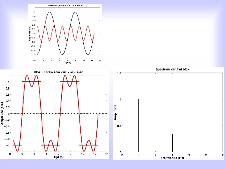
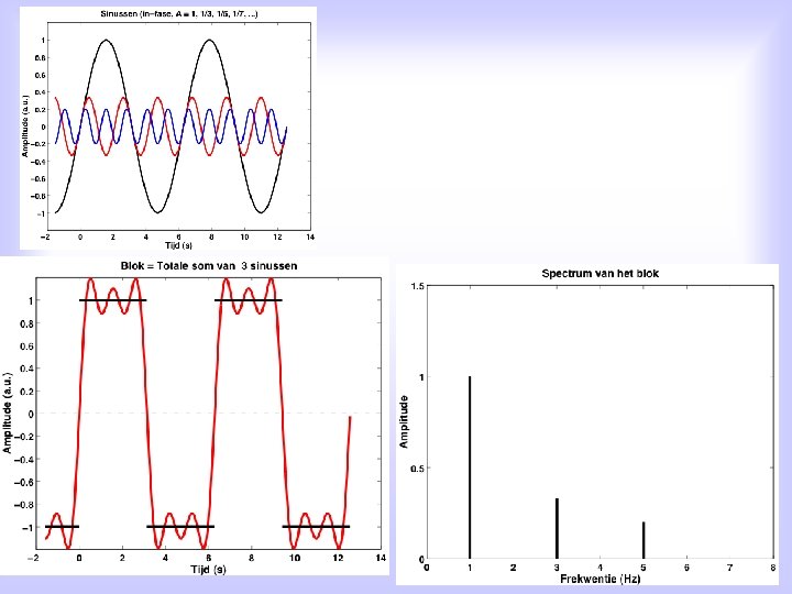
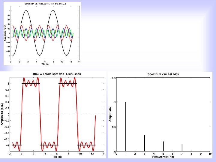
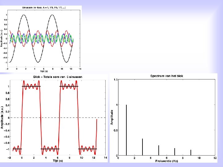
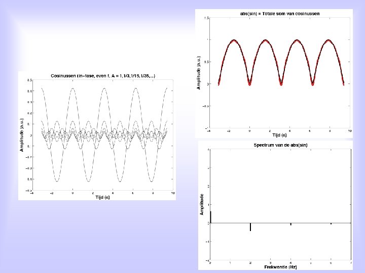
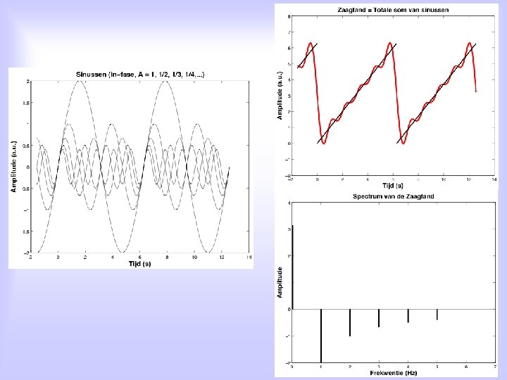
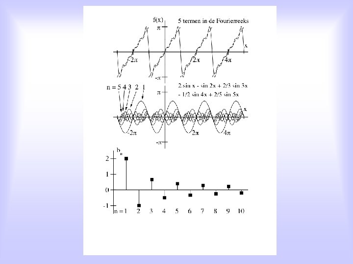
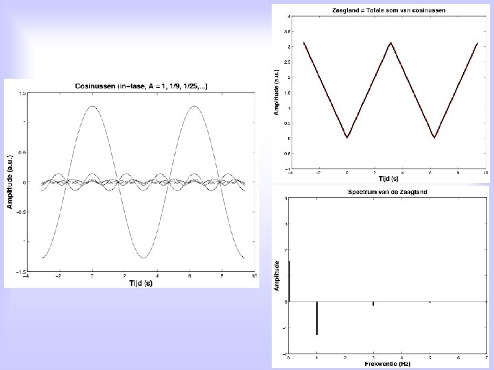
Alternative: For EACH periodic function, x(t), with period T 0, holds: Signal x(t) can be written as a sum of elementary harmonic functions, i. e. sines and cosines, with each sine/cosine its own frequency, which is an integer multiple of the signal’s groundfrequency, and its own amplitude: an en bn are the so-called Fourier coefficients n=1, 2, 3, 4, . . . is the spectral number, and fo is de ground frequency of the signal T 0 is the signal’s period

Fourier-series written slightly differently: amplitude phase frequency

EXAMPLE:

Quantitatively: for the Fourier coefficients it can be proven that: With this in mind, we can now compute the Fourier coefficients ourselves for some simple examples.

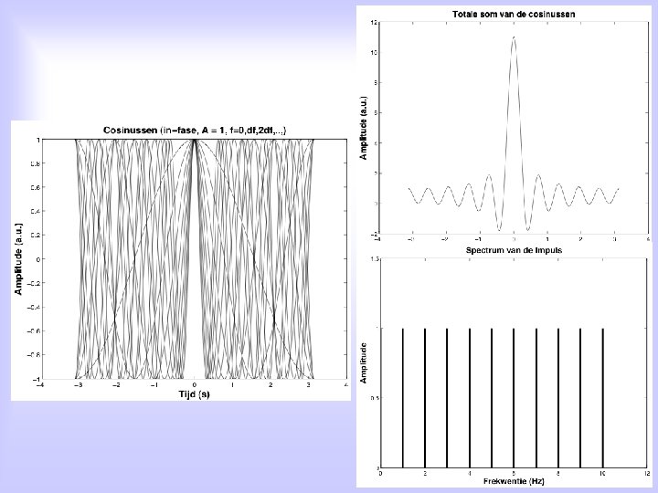
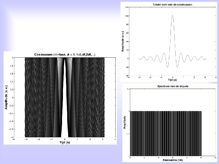
Fourier-analysis on periodic signals: A discrete spectrum: f = n • f 0, met n=1, 2, 3, 4, . . .

short pulse long pulse broad bandwidth narrow bandwidth

shortest slightly longer broad less broad narrower yet longer narrowest longest
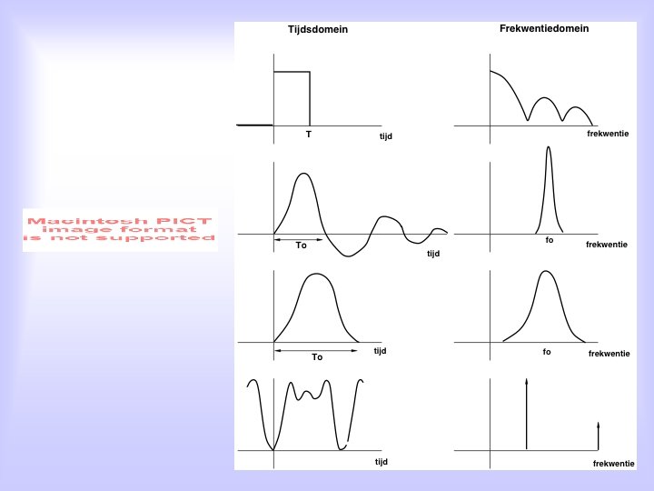

Also non-periodic signals have a Fourier spectrum. In this case, the Fourier series becomes a Fourier integral, for which the period is infinitely long, and the ground frequency (and the frequency interval), df, goes to zero: c(f) is now a continuous amplitude spectrum, and (f) is the continuous phase spectrum of x(t)

End first lecture
- Slides: 37