Atmospheric Science 820 01 Regional Weather and Climate

Atmospheric Science 820. 01 Regional Weather and Climate Modeling: Finite Difference Equations, Vertical Coordinates & Model Grids Sources: Keith Hines Byrd Polar Research Center Wikipedia A. J. Broccoli class notes (http: //www. envsci. rutgers. edu/~broccoli/) Peter Lynch class notes (http: //mathsci. ucd. ie/met/msc/NWP/MAPH-P 313. html) Chris Bretherton class notes (http: //www. atmos. washington. edu/2002 Q 2/547/) Mesoscale Meteorology and Forecasting (Ray) Climate System Modeling (Trenberth) An Introduction to Three-Dimensional Climate Modeling (Washington and Parkinson)

Atmospheric modeling Finite difference Equations Vertical Coordinates Model Grids

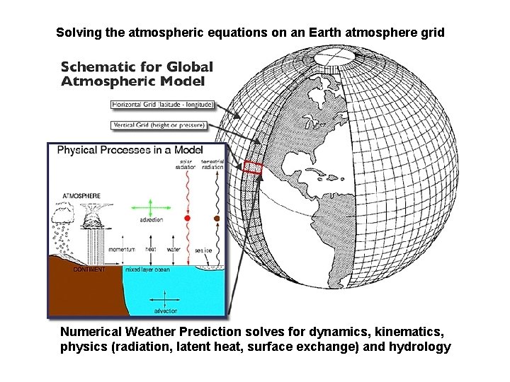
Solving the atmospheric equations on an Earth atmosphere grid Numerical Weather Prediction solves for dynamics, kinematics, physics (radiation, latent heat, surface exchange) and hydrology

Finite Differencing Space Time

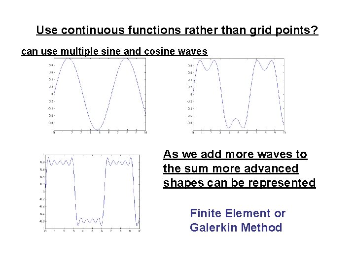
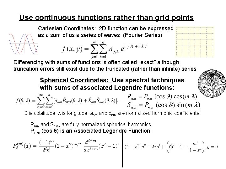
Use continuous functions rather than grid points? can use multiple sine and cosine waves As we add more waves to the sum more advanced shapes can be represented Finite Element or Galerkin Method

Use continuous functions rather than grid points Cartesian Coordinates: 2 D function can be expressed as a sum of as a series of waves (Fourier Series) Differencing with sums of functions is often called “exact” although truncation errors still exist due to the truncated (rather than infinite) series Spherical Coordinates: Use spectral techniques with sums of associated Legendre functions: θ is colatitude, λ is longitude, anm and bnm are normalized harmonic coefficients Rn m and Sn m, are fully normalized spherical harmonics. Pn m (cos θ) is an Associated Legendre Function.

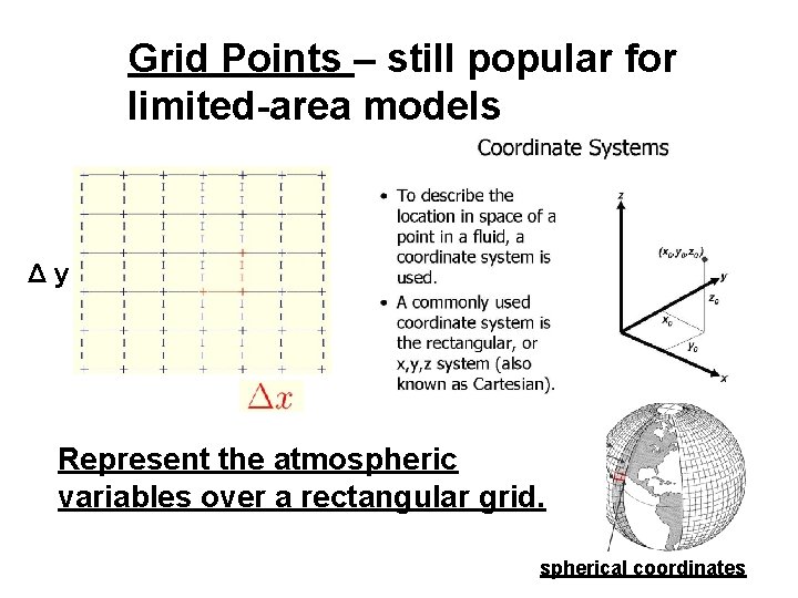
Grid Points – still popular for limited-area models Δy Represent the atmospheric variables over a rectangular grid. spherical coordinates

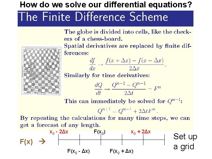
How do we solve our differential equations? x 0 - 2Δx F(x 0) x 0 + 2Δx F(x) F(x 0 - Δx) F(x 0 + Δx) Set up a grid

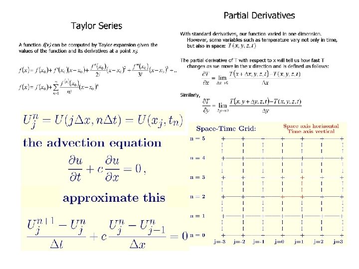
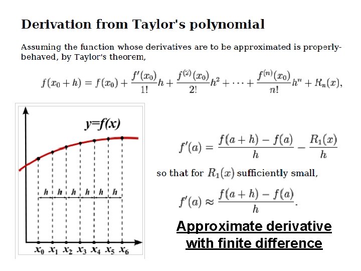
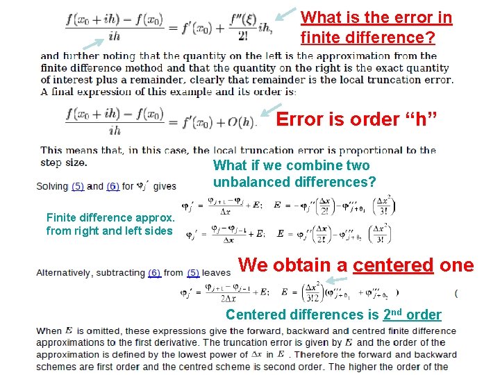
Approximate derivative with finite difference

What is the error in finite difference? Error is order “h” What if we combine two unbalanced differences? Finite difference approx. from right and left sides We obtain a centered one Centered differences is 2 nd order

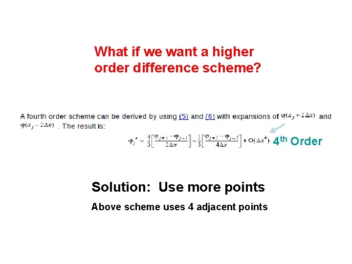
What if we want a higher order difference scheme? 4 th Order Solution: Use more points Above scheme uses 4 adjacent points

Numerical Techniques What do we want in our numerical models? • Accuracy (obvious) • Balance (not dominated by “noise”) • Conservation of key physical properties • Numerical Stability (model survives run) • Efficiency (obvious)

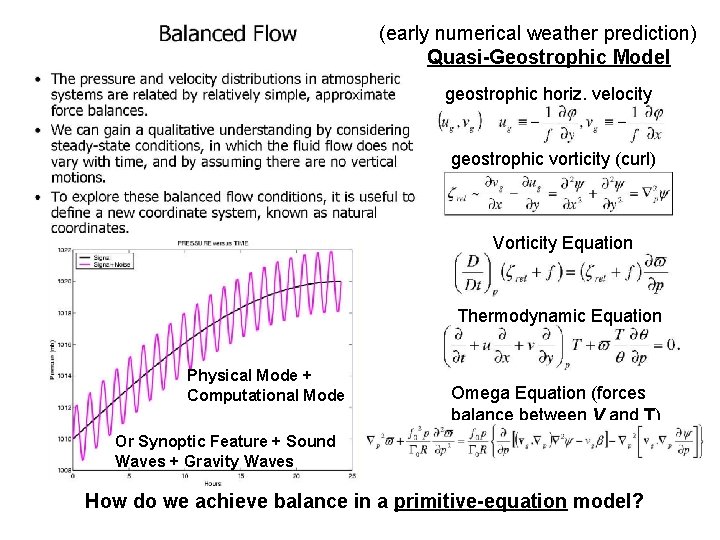
(early numerical weather prediction) Quasi-Geostrophic Model geostrophic horiz. velocity geostrophic vorticity (curl) Vorticity Equation Thermodynamic Equation Physical Mode + Computational Mode Omega Equation (forces balance between V and T) Or Synoptic Feature + Sound Waves + Gravity Waves How do we achieve balance in a primitive-equation model?

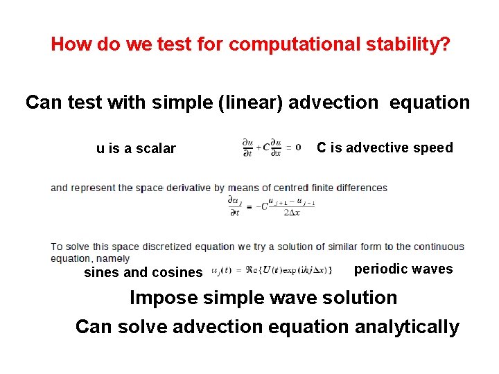
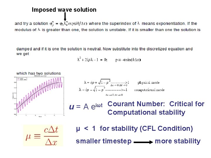
How do we test for computational stability? Can test with simple (linear) advection equation u is a scalar sines and cosines C is advective speed periodic waves Impose simple wave solution Can solve advection equation analytically

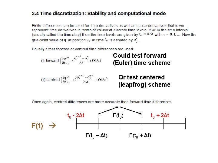
Could test forward (Euler) time scheme Or test centered (leapfrog) scheme t 0 - 2Δt F(t 0) t 0 + 2Δt F(t) F(t 0 – Δt) F(t 0 + Δt)

Imposed wave solution u = A eiωt Courant Number: Critical for Computational stability μ < 1 for stability (CFL Condition) smaller timestep more stability

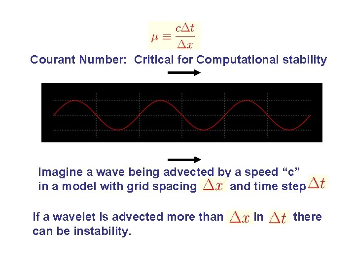
Courant Number: Critical for Computational stability Imagine a wave being advected by a speed “c” in a model with grid spacing and time step If a wavelet is advected more than can be instability. in there

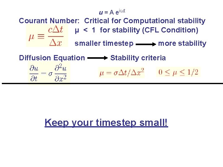
u = A eiωt Courant Number: Critical for Computational stability μ < 1 for stability (CFL Condition) smaller timestep Diffusion Equation more stability Stability criteria Keep your timestep small!

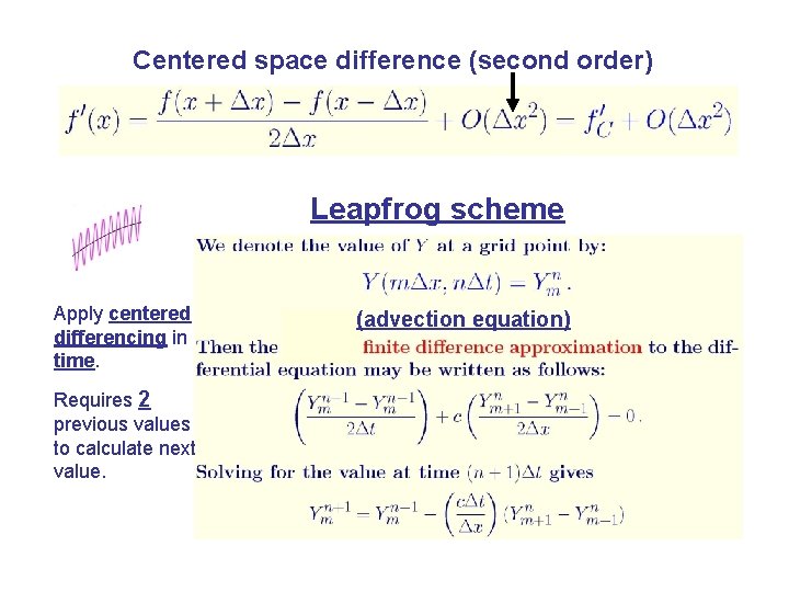
Centered space difference (second order) Leapfrog scheme Apply centered differencing in time. Requires 2 previous values to calculate next value. (advection equation)

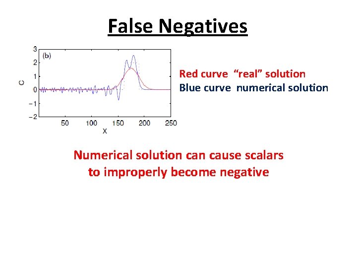
False Negatives Red curve “real” solution Blue curve numerical solution Numerical solution cause scalars to improperly become negative

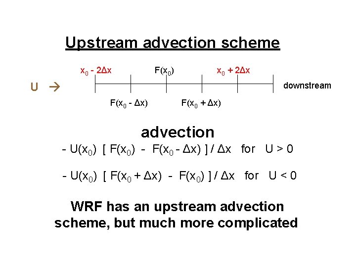
Upstream advection scheme x 0 - 2Δx F(x 0) x 0 + 2Δx U downstream F(x 0 - Δx) F(x 0 + Δx) advection - U(x 0) [ F(x 0) - F(x 0 - Δx) ] / Δx for U > 0 - U(x 0) [ F(x 0 + Δx) - F(x 0) ] / Δx for U < 0 WRF has an upstream advection scheme, but much more complicated

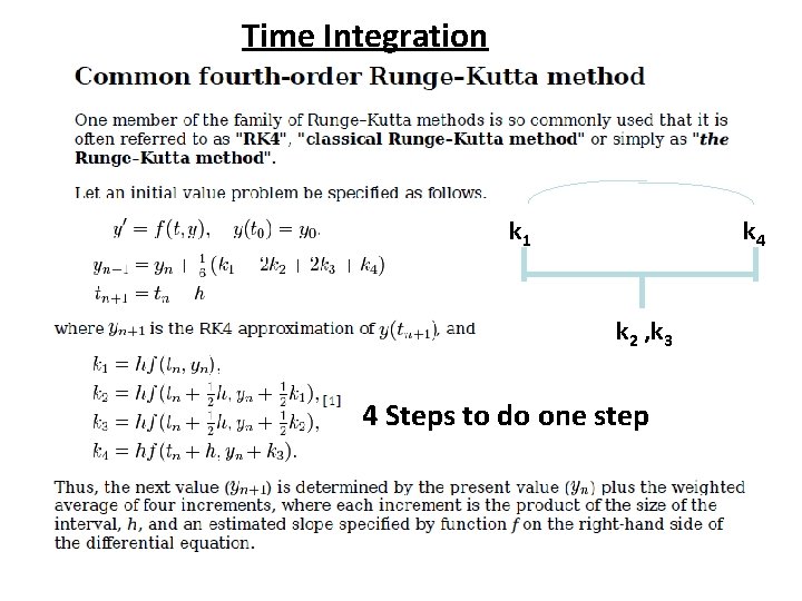
Time Integration k 1 k 4 k 2 , k 3 4 Steps to do one step

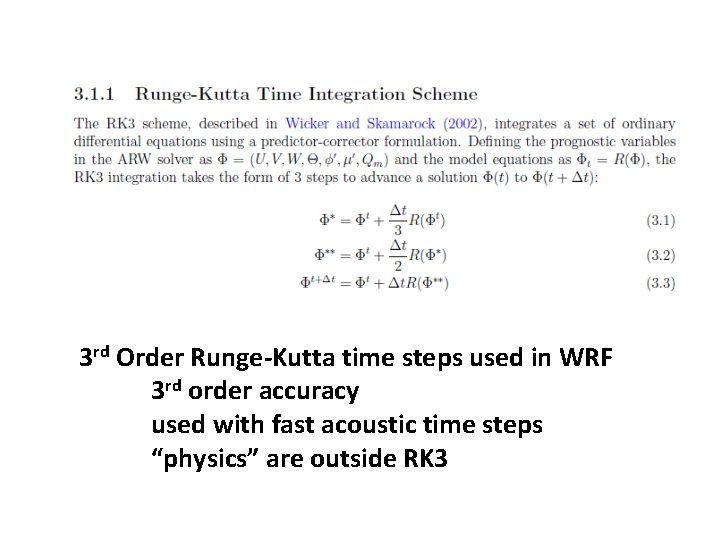
3 rd Order Runge-Kutta time steps used in WRF 3 rd order accuracy used with fast acoustic time steps “physics” are outside RK 3

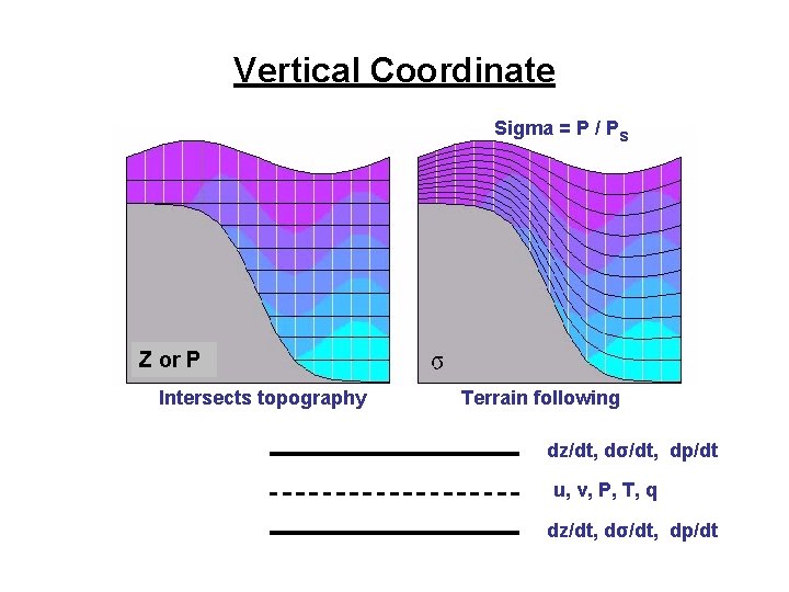
Vertical Coordinate Sigma = P / Ps Z or P Intersects topography Terrain following dz/dt, dσ/dt, dp/dt u, v, P, T, q dz/dt, dσ/dt, dp/dt

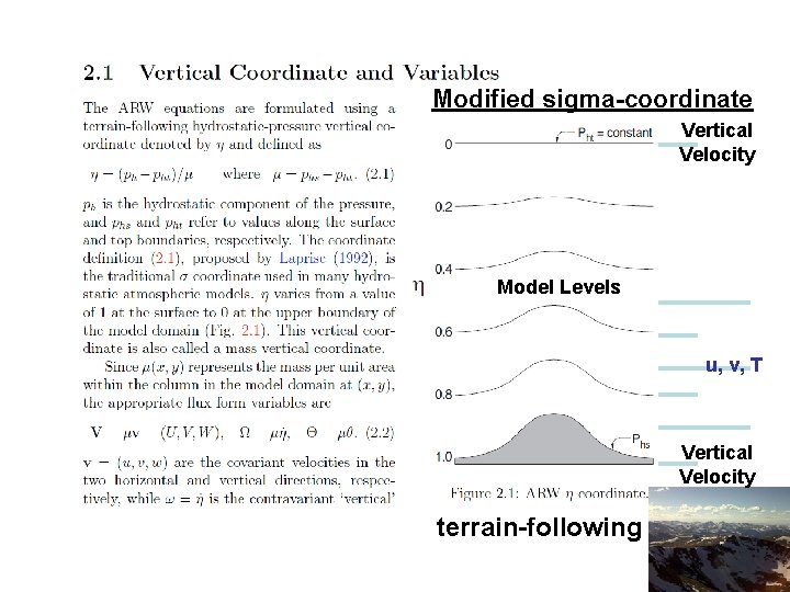
Modified sigma-coordinate Vertical Velocity Model Levels u, v, T Vertical Velocity terrain-following

Numerical Techniques: Grids

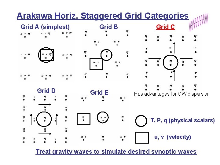
Arakawa Horiz. Staggered Grid Categories Grid A (simplest) Grid D Grid B Grid E Grid C Has advantages for GW dispersion T, P, q (physical scalars) u, v (velocity) Treat gravity waves to simulate desired synoptic waves

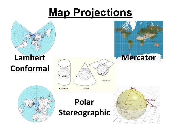
Map Projections Mercator Lambert Conformal Polar Stereographic

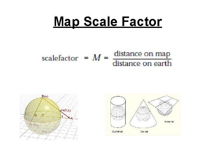
Map Scale Factor

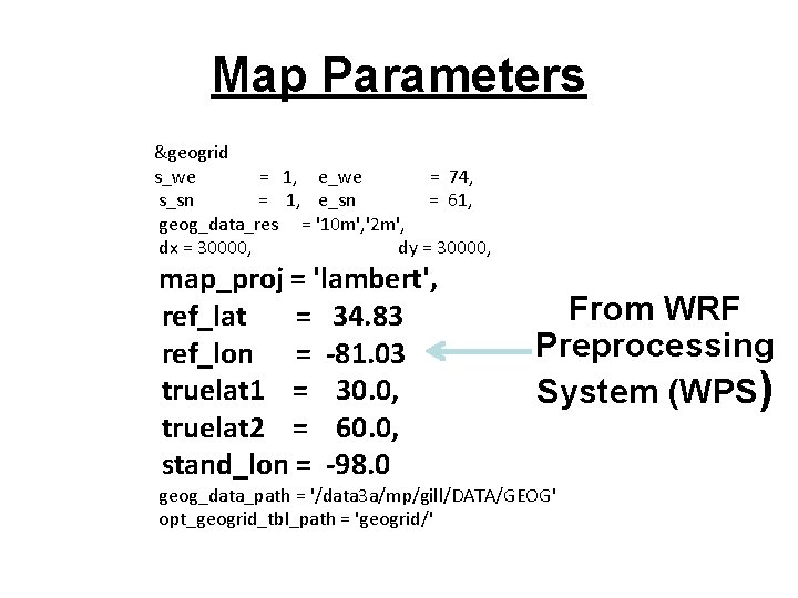
Map Parameters &geogrid s_we = 1, e_we = 74, s_sn = 1, e_sn = 61, geog_data_res = '10 m', '2 m', dx = 30000, dy = 30000, map_proj = 'lambert', ref_lat = 34. 83 ref_lon = -81. 03 truelat 1 = 30. 0, truelat 2 = 60. 0, stand_lon = -98. 0 From WRF Preprocessing System (WPS) geog_data_path = '/data 3 a/mp/gill/DATA/GEOG' opt_geogrid_tbl_path = 'geogrid/'

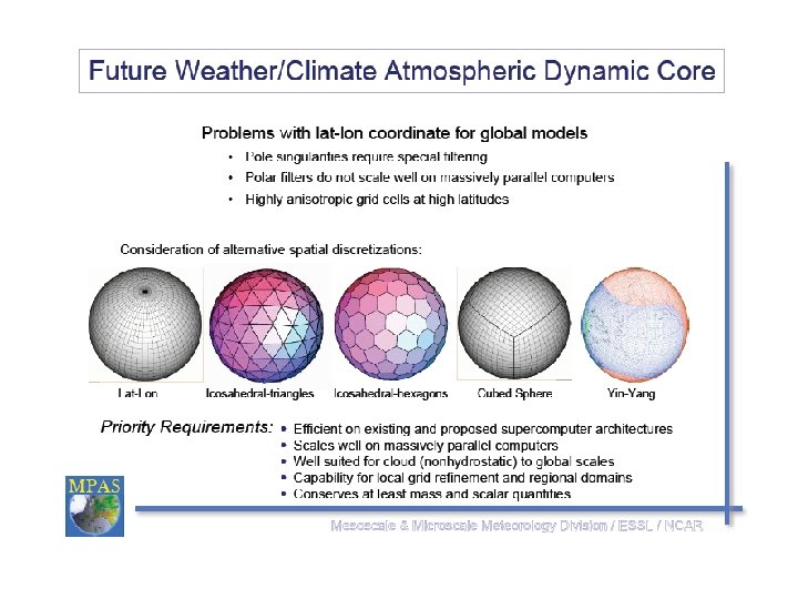
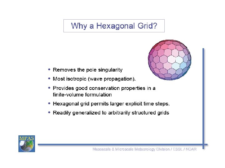
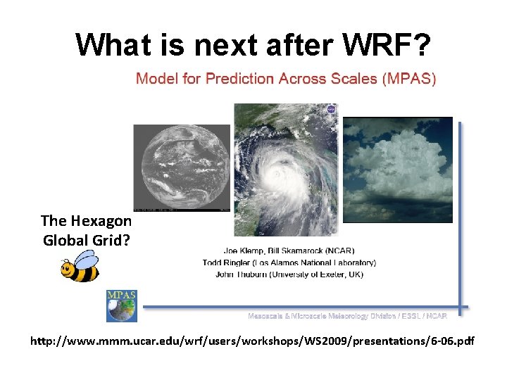
What is next after WRF? The Hexagon Global Grid? http: //www. mmm. ucar. edu/wrf/users/workshops/WS 2009/presentations/6 -06. pdf