Atmospheric Dispersion AD 1 Outline Eulerian approach Lagrangian

Atmospheric Dispersion (AD) 1

Outline • Eulerian approach • Lagrangian approach eqns for mean concentration, solutions for instantaneous and continuous source • Gaussian plume eqn AD parameterizations (P-G curves), plume rise 2

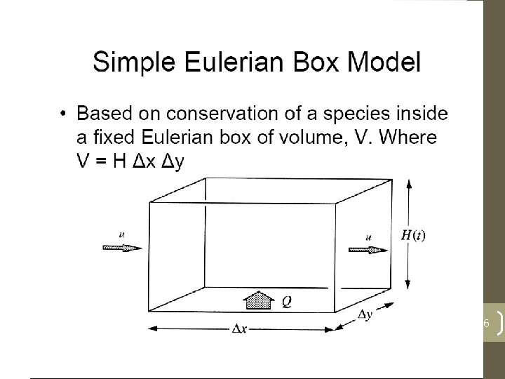
Air pollution dispersion models • Box model air pollutants inside the box are homogeneously distributed • Gaussian model is perhaps the oldest (circa 1936) • Lagrangian model - statistics of the trajectories of a large number of the pollution plume parcels. • Eulerian model - fixed three-dimensional Cartesian grid • Dense gas model • Hybrids (Plume in Grid model) 3

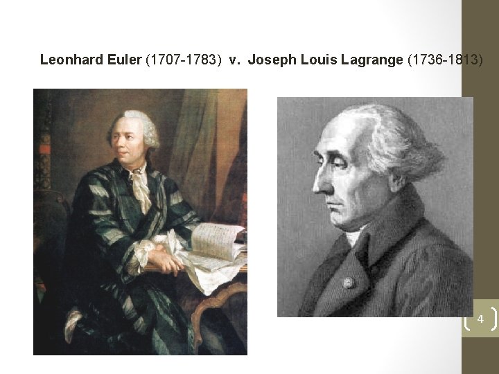
Leonhard Euler (1707 -1783) v. Joseph Louis Lagrange (1736 -1813) 4

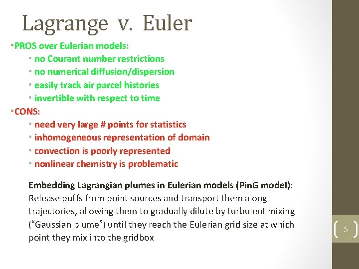
Lagrange v. Euler • PROS over Eulerian models: • no Courant number restrictions • no numerical diffusion/dispersion • easily track air parcel histories • invertible with respect to time • CONS: • need very large # points for statistics • inhomogeneous representation of domain • convection is poorly represented • nonlinear chemistry is problematic Embedding Lagrangian plumes in Eulerian models (Pin. G model): Release puffs from point sources and transport them along trajectories, allowing them to gradually dilute by turbulent mixing (“Gaussian plume”) until they reach the Eulerian grid size at which point they mix into the gridbox 5

6

7

Eulerian approach 8

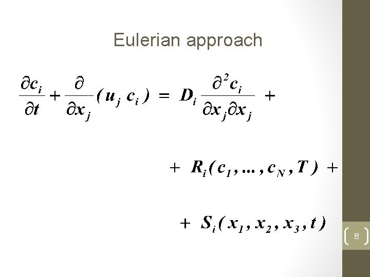
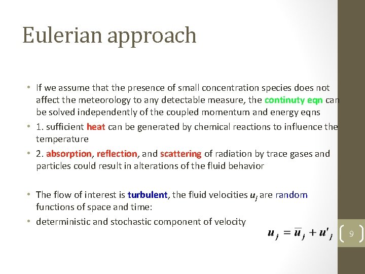
Eulerian approach • If we assume that the presence of small concentration species does not affect the meteorology to any detectable measure, the continuty eqn can be solved independently of the coupled momentum and energy eqns • 1. sufficient heat can be generated by chemical reactions to influence the temperature • 2. absorption, reflection, and scattering of radiation by trace gases and particles could result in alterations of the fluid behavior • The flow of interest is turbulent, the fluid velocities uj are random functions of space and time: • deterministic and stochastic component of velocity 9

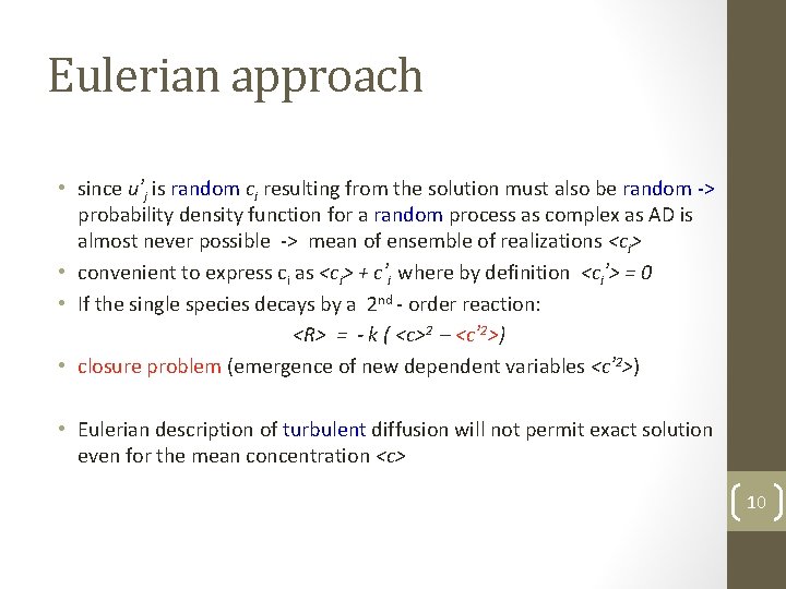
Eulerian approach • since u’j is random ci resulting from the solution must also be random -> probability density function for a random process as complex as AD is almost never possible -> mean of ensemble of realizations <ci> • convenient to express ci as <ci> + c’i where by definition <ci’> = 0 • If the single species decays by a 2 nd - order reaction: <R> = - k ( <c>2 – <c’ 2>) • closure problem (emergence of new dependent variables <c’ 2>) • Eulerian description of turbulent diffusion will not permit exact solution even for the mean concentration <c> 10

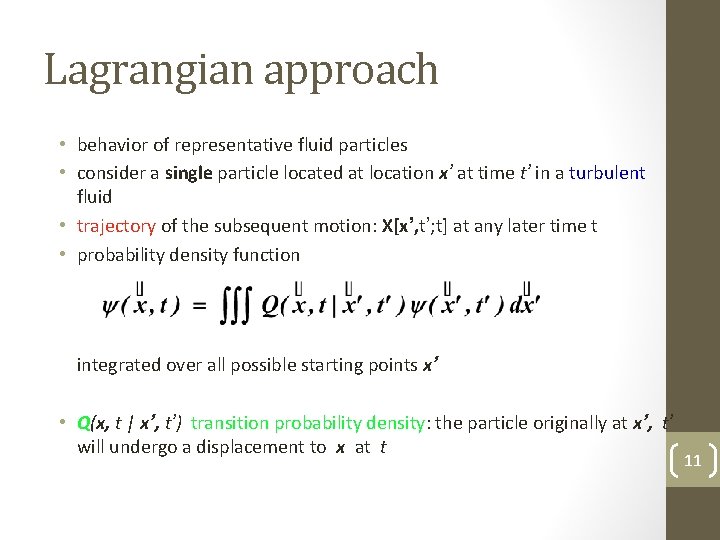
Lagrangian approach • behavior of representative fluid particles • consider a single particle located at location x’ at time t’ in a turbulent fluid • trajectory of the subsequent motion: X[x’, t’; t] at any later time t • probability density function integrated over all possible starting points x’ • Q(x, t | x’, t’) transition probability density: the particle originally at x’, t’ will undergo a displacement to x at t 11

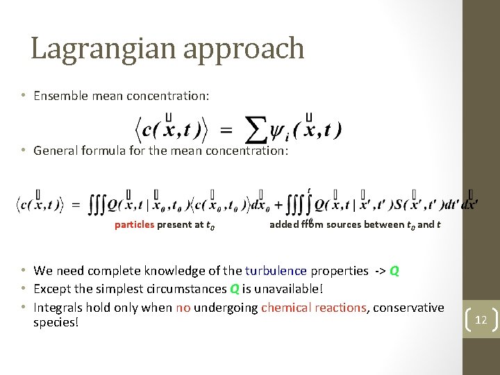
Lagrangian approach • Ensemble mean concentration: • General formula for the mean concentration: particles present at t 0 added from sources between t 0 and t • We need complete knowledge of the turbulence properties -> Q • Except the simplest circumstances Q is unavailable! • Integrals hold only when no undergoing chemical reactions, conservative species! 12

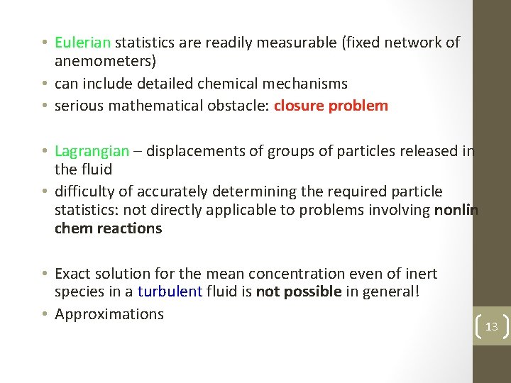
• Eulerian statistics are readily measurable (fixed network of anemometers) • can include detailed chemical mechanisms • serious mathematical obstacle: closure problem • Lagrangian – displacements of groups of particles released in the fluid • difficulty of accurately determining the required particle statistics: not directly applicable to problems involving nonlin chem reactions • Exact solution for the mean concentration even of inert species in a turbulent fluid is not possible in general! • Approximations 13

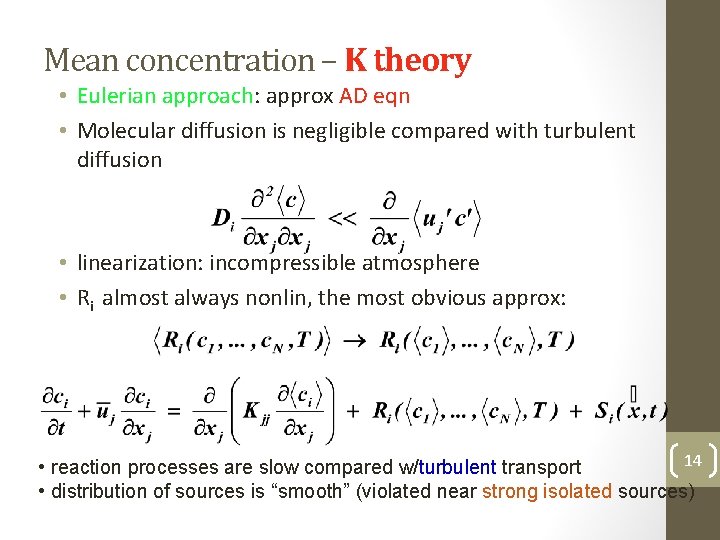
Mean concentration – K theory • Eulerian approach: approx AD eqn • Molecular diffusion is negligible compared with turbulent diffusion • linearization: incompressible atmosphere • Ri almost always nonlin, the most obvious approx: 14 • reaction processes are slow compared w/turbulent transport • distribution of sources is “smooth” (violated near strong isolated sources)

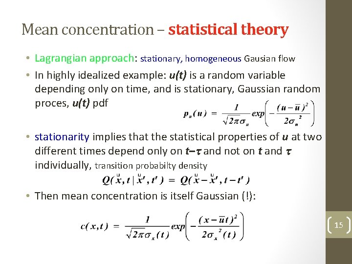
Mean concentration – statistical theory • Lagrangian approach: stationary, homogeneous Gausian flow • In highly idealized example: u(t) is a random variable depending only on time, and is stationary, Gaussian random proces, u(t) pdf • stationarity implies that the statistical properties of u at two different times depend only on t–t and not on t and t individually, transition probabilty density • Then mean concentration is itself Gaussian (!): 15

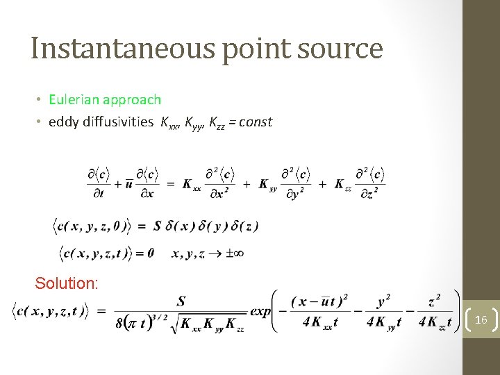
Instantaneous point source • Eulerian approach • eddy diffusivities Kxx, Kyy, Kzz = const Solution: 16

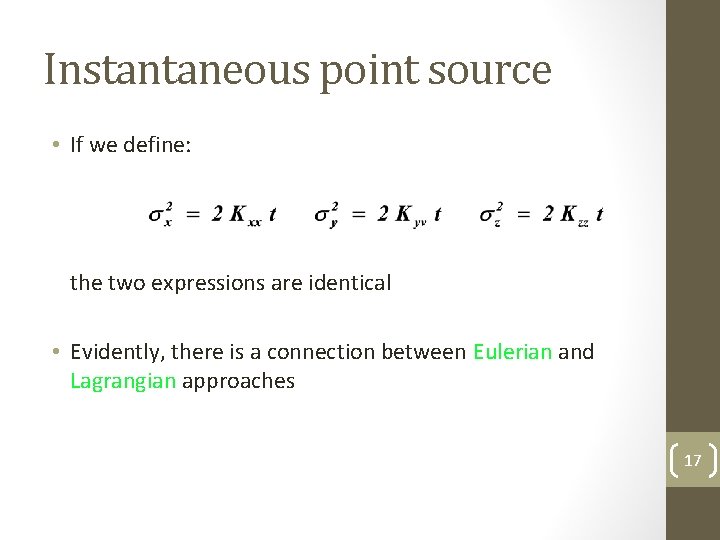
Instantaneous point source • If we define: the two expressions are identical • Evidently, there is a connection between Eulerian and Lagrangian approaches 17

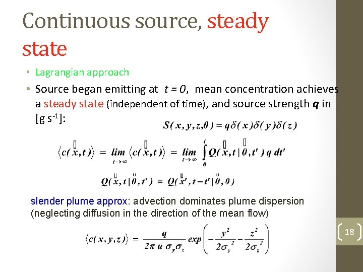
Continuous source, steady state • Lagrangian approach • Source began emitting at t = 0, mean concentration achieves a steady state (independent of time), and source strength q in [g s-1]: slender plume approx: advection dominates plume dispersion (neglecting diffusion in the direction of the mean flow) 18

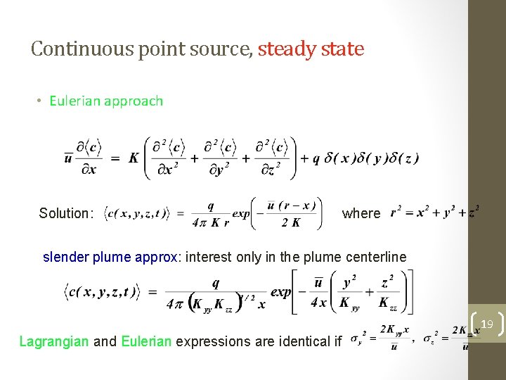
Continuous point source, steady state • Eulerian approach Solution: where slender plume approx: interest only in the plume centerline 19 Lagrangian and Eulerian expressions are identical if

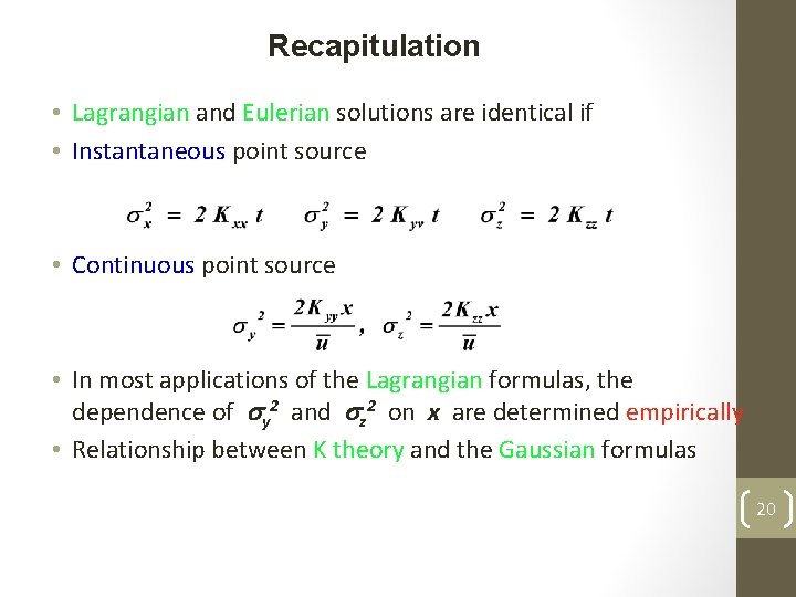
Recapitulation • Lagrangian and Eulerian solutions are identical if • Instantaneous point source • Continuous point source • In most applications of the Lagrangian formulas, the dependence of sy 2 and sz 2 on x are determined empirically • Relationship between K theory and the Gaussian formulas 20

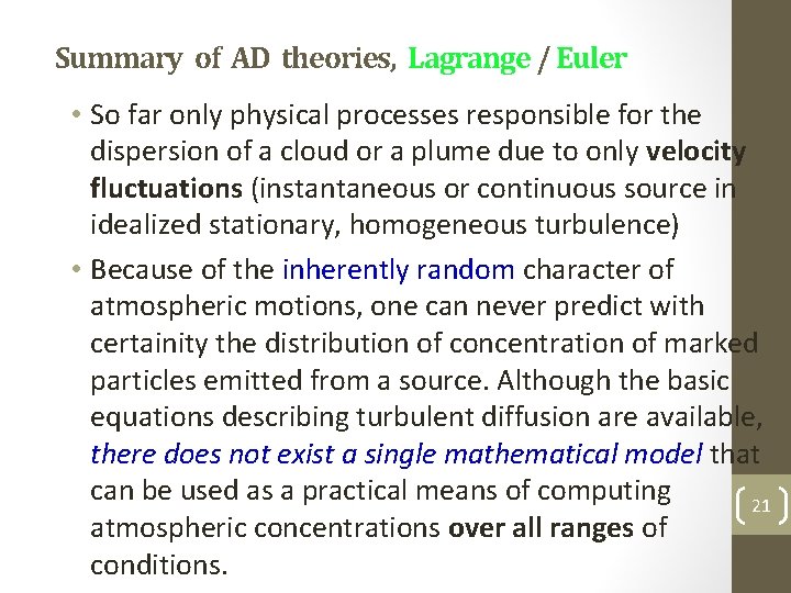
Summary of AD theories, Lagrange / Euler • So far only physical processes responsible for the dispersion of a cloud or a plume due to only velocity fluctuations (instantaneous or continuous source in idealized stationary, homogeneous turbulence) • Because of the inherently random character of atmospheric motions, one can never predict with certainity the distribution of concentration of marked particles emitted from a source. Although the basic equations describing turbulent diffusion are available, there does not exist a single mathematical model that can be used as a practical means of computing 21 atmospheric concentrations over all ranges of conditions.

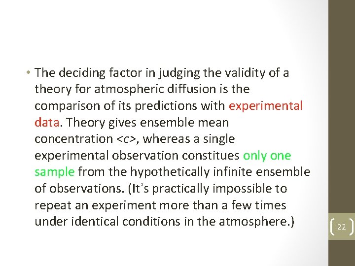
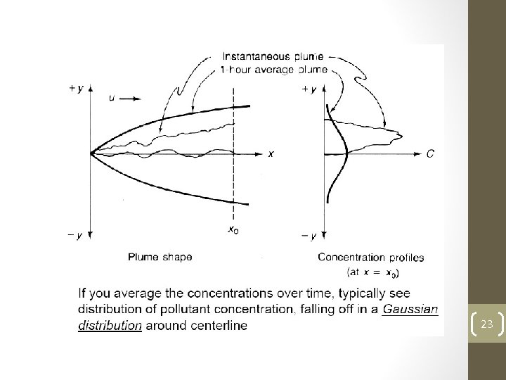
• The deciding factor in judging the validity of a theory for atmospheric diffusion is the comparison of its predictions with experimental data. Theory gives ensemble mean concentration <c>, whereas a single experimental observation constitues only one sample from the hypothetically infinite ensemble of observations. (It’s practically impossible to repeat an experiment more than a few times under identical conditions in the atmosphere. ) 22

23

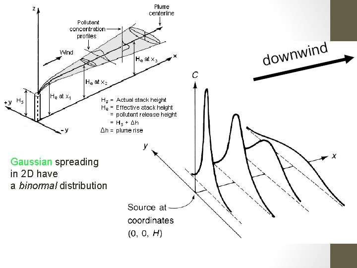
Gaussian spreading in 2 D have a binormal distribution 24

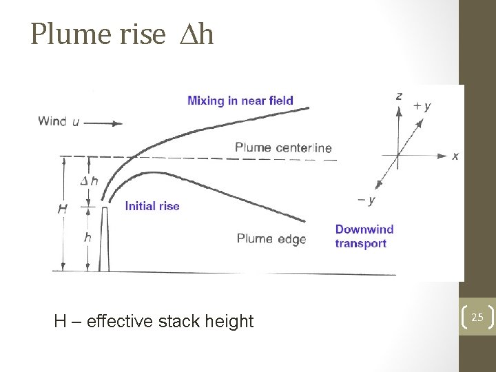
Plume rise Dh H – effective stack height 25

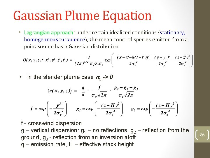
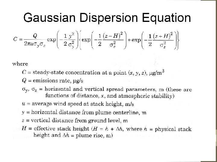
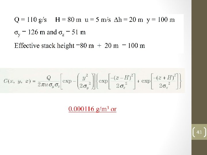
Gaussian Plume Equation • Lagrangian approach: under certain idealized conditions (stationary, homogeneous turbulence), the mean conc. of species emitted from a point source has a Gaussian distribution • in the slender plume case sx -> 0 f - crosswind dispersion g – vertical dispersion: g 1 – no reflections, g 2 – reflection from the ground, g 3 - reflection from an inversion aloft q – emission rate, H – effective stack height 26

27

Gaussian Plume Equation • Eulerian approach: It can be shown (use of Green function) that we can get to the same result by solving the AD eqn (but with const eddy diffusivities)! Johann Carl Friedrich Gauss (1777 -1855) 28

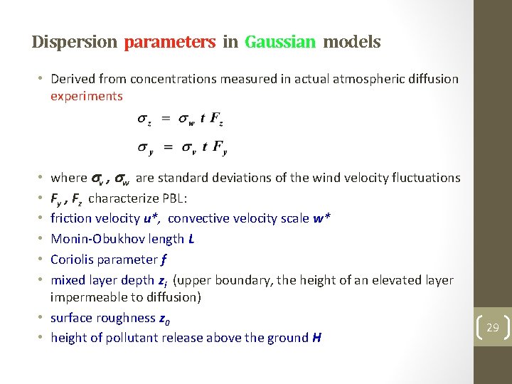
Dispersion parameters in Gaussian models • Derived from concentrations measured in actual atmospheric diffusion experiments where sv , sw are standard deviations of the wind velocity fluctuations Fy , Fz characterize PBL: friction velocity u*, convective velocity scale w* Monin-Obukhov length L Coriolis parameter f mixed layer depth zi (upper boundary, the height of an elevated layer impermeable to diffusion) • surface roughness z 0 • height of pollutant release above the ground H • • • 29

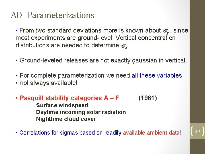
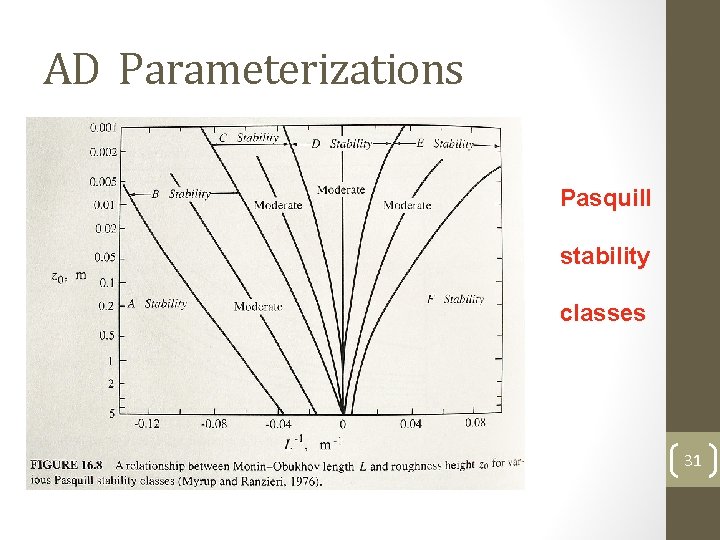
AD Parameterizations • From two standard deviations more is known about sy , since most experiments are ground-level. Vertical concentration distributions are needed to determine sz • Ground-leveled releases are not exactly gaussian in vertical. • For complete parameterization we need all these variables • not always available! • Pasquill stability categories A – F (1961) Surface windspeed Daytime incoming solar radiation Nighttime cloud cover • Correlations for sigmas based on readily available ambient data! 30

AD Parameterizations Pasquill stability classes 31

Pasquill-Gifford (P-G) curves Horizontal and vertical dispersion coeff 32 Distance from source [m]

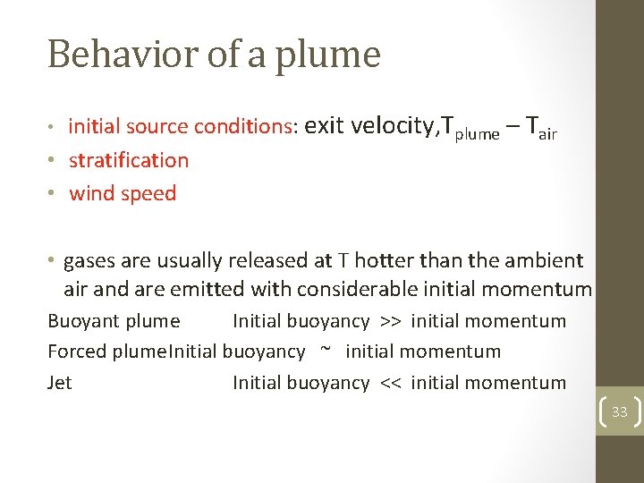
Behavior of a plume • initial source conditions: exit velocity, Tplume – Tair • stratification • wind speed • gases are usually released at T hotter than the ambient air and are emitted with considerable initial momentum Buoyant plume Initial buoyancy >> initial momentum Forced plume. Initial buoyancy ~ initial momentum Jet Initial buoyancy << initial momentum 33

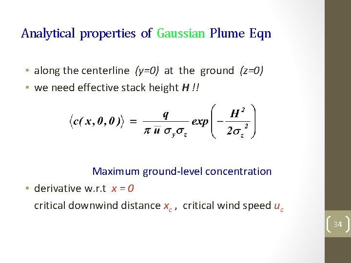
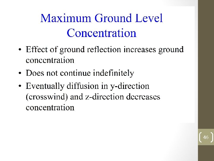
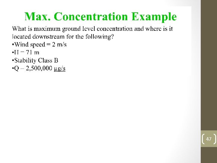
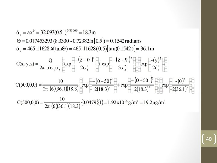
Analytical properties of Gaussian Plume Eqn • along the centerline (y=0) at the ground (z=0) • we need effective stack height H !! Maximum ground-level concentration • derivative w. r. t x = 0 critical downwind distance xc , critical wind speed uc 34

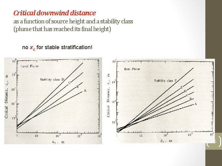
Critical downwind distance as a function of source height and a stability class (plume that has reached its final height) no xc for stable stratification! 35

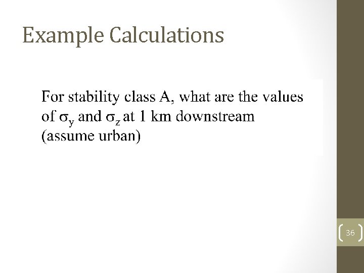
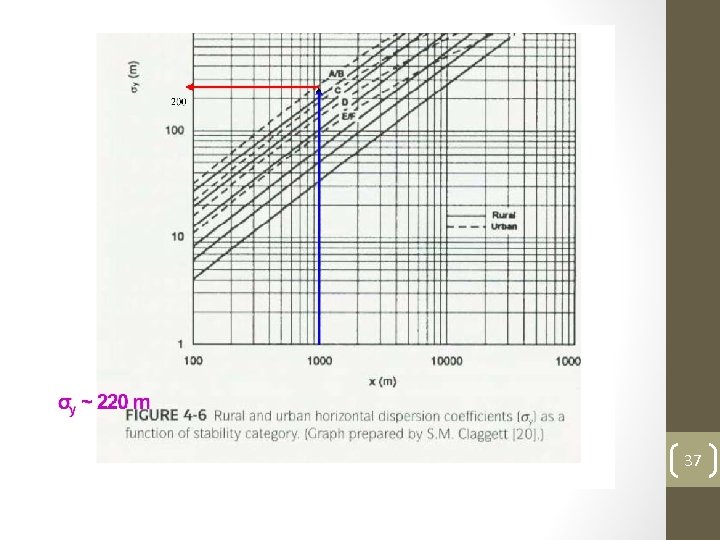
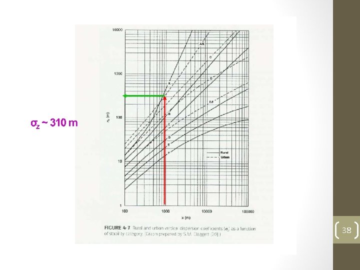
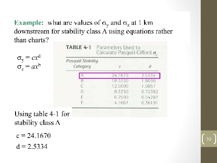
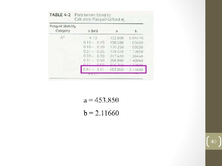
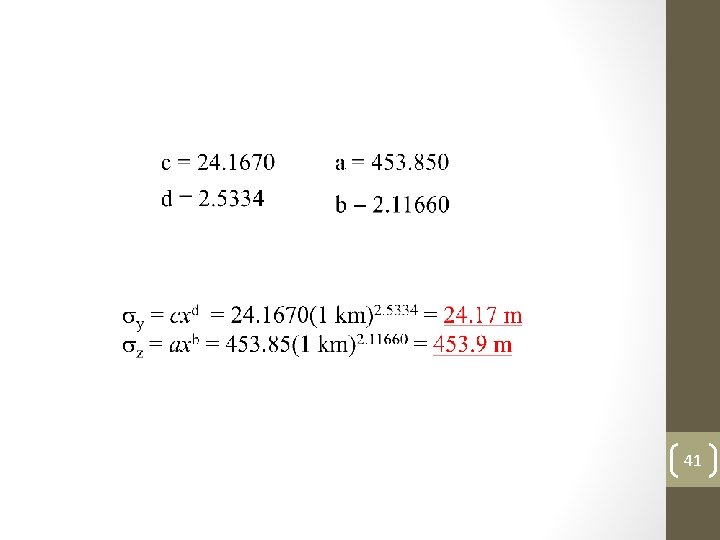
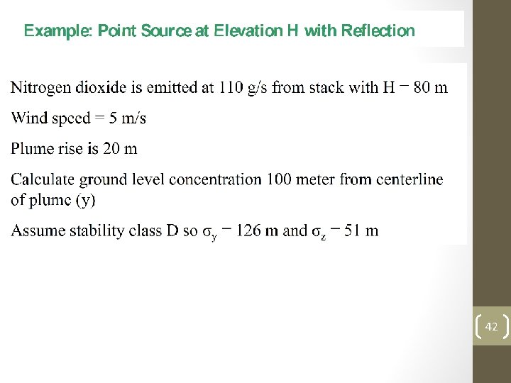
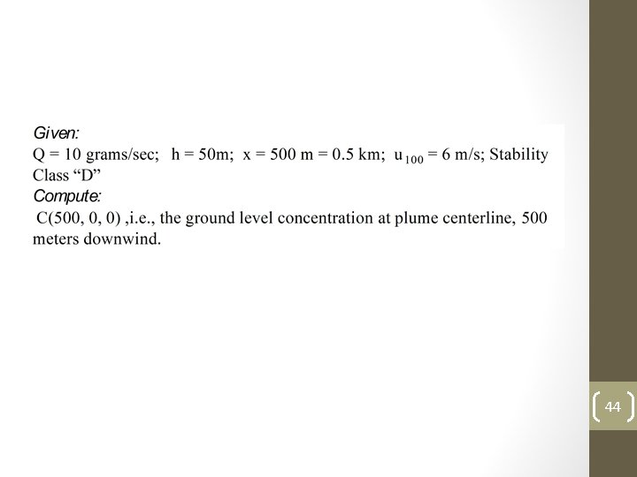
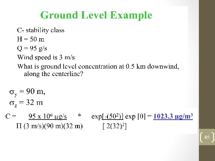
Example Calculations 36

37

38

39

40

41

42

43

44

45

46

47

48