AT 650 Measurements and Instruments Course Objective To

AT 650: Measurements and Instruments • Course Objective: To introduce the student to the practice of measurement providing them with an understanding of basic measurement principles and instrumentation commonly used to observe the atmosphere. I often say that when you can measure what you are speaking about, and express it in numbers, you know something about it; but when you cannot measure it, when you cannot express it in numbers, your knowledge is of a meager and unsatisfactory kind; it may be the beginning of knowledge, but you have scarcely, in your thoughts, advanced to the stage of science, whatever the matter may be. Lord Kelvin

• Class Organization & Schedule: • Assessment: 4 class projects • Rawinsonde project • Interferometer analysis • Measurement design/execution (urban heat island) • Field Experiment design (clouds/aerosols) • Class participation and attendance If you must miss class for more than a lecture, can make up via short report on topic related to class. Arranged individually.

• Schedule - flexible to accommodate a number of guest lectures from instrument experts and some experiements that take longer than 50 min. • August • 23/25: Introduction and background • Aug 30: Richard Austin - Temperature measurements • Sept 1: Error estimation • September: In-situ surface and upper air observations • October: Radiometric observations (passive) • November: Radiometric observations (active) • Dec: Reports on Field Experiments

1. 0 Background to Observing systems input Measurement system Z(t) T y(t) y = F(Z, b, c) + System (nature’s) forward function y f(Z, b) + y + f Z = f-1(y, b) system inverse function Focus of this class output Z(t) T The ‘system’ • measurement y • forward model f • parameters b • Assumptions, c • errors, y + f

Suppose Z(t) is the true rainfall rate [mm/hr]. We are trying to measure it with a bucket sitting on a scale whose weight is recorded every hour. Z(t) T y(t) y = F(Z, b, c) + y = weight of scale y = uncertainty of weight measurement b 1 = opening of bucket exposed to rain b 2 = weight of empty bucket c = all those other little things c 1 = wind speed c 2 = dead bugs in bucket y f(Z, b) + y + f Z = f-1(y, b) Z(t) T Z = f-1(y, b) is the derived rainfall. It is explicitly computed in this case. z = the uncertainty. Explicit from y + f but not from inverse of c All the difficulty is in “c” or “ f ” which is not necessarily random

Assessment of Uncertainties of Measurements National Association of testing Authorities, under the auspices of the International Organization for Standards (ISO) - Guide to the expression of uncertainty in Measurements (ISO-GUM) ISO GUM recommends that individual uncertainties be estimated via type A or type B evaluation. Type A involves analysis of data via established statistical methods, Type B uses other means, including for e. g. a priori knowledge. There are two types of uncertainty – random and systematic

Sources/components of Uncertainty: Random variation can occur for several reasons – they could be a function of the measurement environment (e. g. temperature fluctuations, other factors out of the control Random errors are an inevitable element of any measurement system These are evaluated using statistical means (type A analyses)

Elements of a simple measurement system: input transducer V 1 Analog signal conditioner V 2 Calibration converts V 3 to y Analog to digital Sensor that converts one form of energy to another (e. g. radiation to voltage) Amplifiers for gain and offset, filters to reduce noise, etc This conversion can add (digitizer) noise V 3 Digital processing, data archival, display Microprocessors, hard drives Tape drives, software analyses etc, etc

Sources/components of Uncertainty: Systematic The bane of any measurement exercise – it is a characteristic of systematic errors that the magnitude and sign can neither be reduced or knowledge improved by averaging repeated measurements. Measurement y r c i t a m e t s Sy True y ro r e random error (precision) Because systematic errors do not change under fixed conditions, they are difficult to detect

Random vs Systematic uncertainties In real life, the two components almost always coexist. The relative magnitude depends largely upon space and time averaging of measurement.

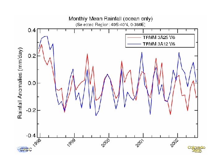
PR/TMI Rainfall Differences (5 -year mean PR-2 A 25 - TMI-2 A 12 from 3 G 68)

1. 1 The Measurand its range Measurand – quantity subject to measurement. This cannot be known exactly. Every measurement has an error attached to it and without a quantitative statement of error, measurements lack worth For atmospheric sciences, • State of the atmosphere (pressure, temperature, gaseous concentrations – water vapor, ozone, clouds, precipitation ) • Motions of the atmosphere (wind speed, direction, vertical motions) • external influences on the atmosphere – radiative & turbulent fluxes, etc Range – measurand interval over which sensor is calibrated

The example of the Automated Surface Observing System (ASOS)

Sources of error

Under the ISO GUM, uncertainty is stated wrt the 95% confidence level. Why the 95% confidence level: • Established practice world-wide • The ISO guide assumes that the combined uncertainty is close to normally distributed. It is a general belief that most measurement systems more or less approximate to a normal distribution out to two standard deviations • The 95% confidence interval can be simply approximated by multiplying the SD by a factor of 2.

1. 2 Instrument Types: (i) in situ or immersion instruments –the response of the instrument is directly related to the measurand (ii) remote sensing instruments –these instruments provide measurements of quantities indirectly related to the quantity of interest passive Furthermore, there are two types of remote Sensing instruments – active & passive active

1. 3 Terminologies Quantity- particular attribute of a phenomenon Value- magnitude of a quantity (ie a number) True Value – value consistent with definition of quantity – hypothetical and cannot be measured but can be approached (incrementally) using ‘more accurate’ measurement systems. Measurement – set of operations with a goal to determine value of a quantity Influence quantity – quantity not measurable but affects result of measurement

Sensor: An element that receives energy associated with the measured quantity and produces an output signal associated in some way to the measurand. The sensor always adds a little noise making a perfect measurement theoretically impossible A variety of different detector types, their spectral ranges and sensitivities.

Accuracy – closeness of agreement between the result of a measurement and true value of the measurand Repeatability –closeness of agreement between the results of a measurement under the same conditions (which must be specified) Reproducibility - closeness of agreement between the results of a measurement under the different conditions (which must be specified) Uncertainty – a parameter associated with a set of measurements that characterizes the dispersion of values reasonably attributed to the measurand – there are two types of uncertainty evaluations type A: evaluated using statistical means type B: evaluated using other means, like knowledge & experience

Calibration: Conversion of the output of the sensor to a physical quantity. Ideally this conversion should be performed wrt a traceable standard. Static Calibration: the measurements are performed under ‘steady-state’ conditions where output is steady. Vicarious Calibration: calibration against a non-standard reference (source) (e. g. calibration of a radiometer using reflectance from a bright surface)

Calibration (cont’d): output Transfer plot Sensor transfer – input-to-output translation Span – numerical value of range Static Sensitivity – slope of ‘transfer plot’ Resolution – the smallest change in the primary input that produces a detectable change in output Linearity- the degree to which the transfer plot is linear – residual error Hysteresis – sensor output for a given input depends on whether the input is increasing or decreasing. Stability – closeness of repeated calibrations over a period of time input

Calibration (cont’d): Example of Vicarious calibration Albedo derived from AVHRR channel 1 over the southeastern portion of the Libyan desert. Vicarious calibration is necessary for instruments on satellites that do not carry calibration systems on board and suffer from life-time degradation.

Science: Published online 11 August 2005 Reports Submitted on May 12, 2005 Accepted on July 27, 2005 The Effect of Diurnal Correction on Satellite-Derived Lower Tropospheric Temperature Carl A. Mears 1 and Frank J. Wentz 1 1 Remote Sensing Systems, Santa Rosa, CA 94501, USA. Satellite-based measurements of decadal-scale temperature change in the lower troposphere have indicated cooling relative to the surface in the tropics. Such measurements need a diurnal correction to prevent drifts in the satellites' measurement time from causing spurious trends. We have derived a diurnal correction that, in the tropics, is of the opposite sign from that previously applied. When we use this correction in the calculation of lower tropospheric temperature from satellite microwave measurements, we find tropical warming consistent with to that found in surface temperature and in our satellite-derived version of middle/upper tropospheric temperature.

Error- result of measurement minus true value Random Error- result of measurement minus the mean that would result from an infinite number of measurements of the same measurand carried out under repeatable conditions Systematic Error- mean that would result from an infinite number of measurements of the same measurand carried out under repeatable conditions minus the true value of the measurand. Correction- value added to the uncorrected result of measurement to compensate for the systematic error. Uncorrected result- result of measurement before correction for systematic error Corrected result- systematic error removed