Aswath Damodaran 1 VALUATION PACKET 2 RELATIVE VALUATION

Aswath Damodaran 1 VALUATION: PACKET 2 RELATIVE VALUATION, ASSET-BASED VALUATION AND PRIVATE COMPANY VALUATION 1/5/17 Aswath Damodaran Updated: January 2017

The Essence of Relative Valuation (Pricing) 2 In relative valuation, the value of an asset is compared to the values assessed by the market for similar or comparable assets. To do relative valuation then, we need to identify comparable assets and obtain market values for these assets convert these market values into standardized values, since the absolute prices cannot be compared This process of standardizing creates price multiples. compare the standardized value or multiple for the asset being analyzed to the standardized values for comparable asset, controlling for any differences between the firms that might affect the multiple, to judge whether the asset is under or over valued Aswath Damodaran 2

Relative valuation is pervasive… 3 Most asset valuations are relative. Most equity valuations on Wall Street are relative valuations. Almost 85% of equity research reports are based upon a multiple and comparables. More than 50% of all acquisition valuations are based upon multiples Rules of thumb based on multiples are not only common but are often the basis for final valuation judgments. While there are more discounted cashflow valuations in consulting and corporate finance, they are often relative valuations masquerading as discounted cash flow valuations. The objective in many discounted cashflow valuations is to back into a number that has been obtained by using a multiple. The terminal value in a significant number of discounted cashflow valuations is estimated using a multiple. Aswath Damodaran 3

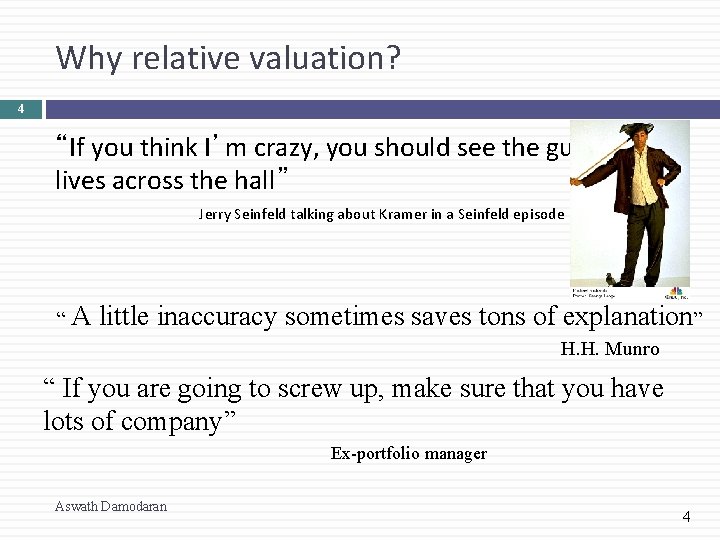
Why relative valuation? 4 “If you think I’m crazy, you should see the guy who lives across the hall” Jerry Seinfeld talking about Kramer in a Seinfeld episode “ A little inaccuracy sometimes saves tons of explanation ” H. H. Munro “ If you are going to screw up, make sure that you have lots of company” Ex-portfolio manager Aswath Damodaran 4

The Market Imperative…. 5 Relative valuation is much more likely to reflect market perceptions and moods than discounted cash flow valuation. This can be an advantage when it is important that the price reflect these perceptions as is the case when the objective is to sell a security at that price today (as in the case of an IPO) investing on “momentum” based strategies With relative valuation, there will always be a significant proportion of securities that are under valued and over valued. Since portfolio managers are judged based upon how they perform on a relative basis (to the market and other money managers), relative valuation is more tailored to their needs Relative valuation generally requires less information than discounted cash flow valuation (especially when multiples are used as screens) Aswath Damodaran 5

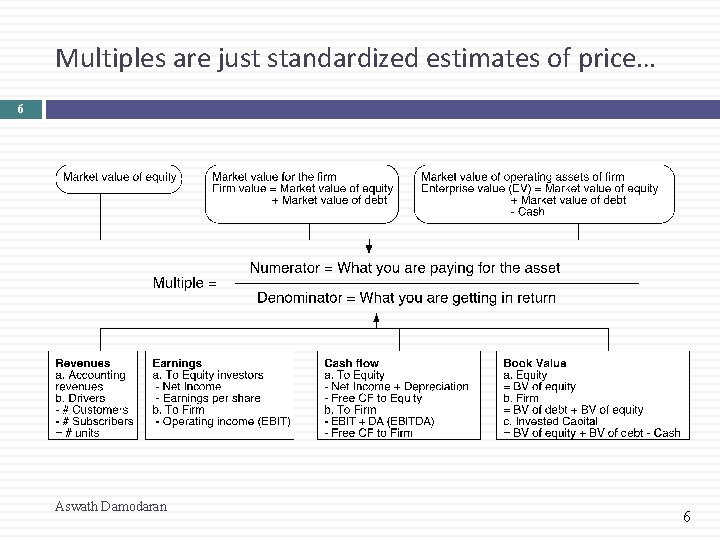
Multiples are just standardized estimates of price… 6 Aswath Damodaran 6

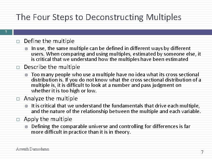
The Four Steps to Deconstructing Multiples 7 Define the multiple Describe the multiple Too many people who use a multiple have no idea what its cross sectional distribution is. If you do not know what the cross sectional distribution of a multiple is, it is difficult to look at a number and pass judgment on whether it is too high or low. Analyze the multiple In use, the same multiple can be defined in different ways by different users. When comparing and using multiples, estimated by someone else, it is critical that we understand how the multiples have been estimated It is critical that we understand the fundamentals that drive each multiple, and the nature of the relationship between the multiple and each variable. Apply the multiple Defining the comparable universe and controlling for differences is far more difficult in practice than it is in theory. Aswath Damodaran 7

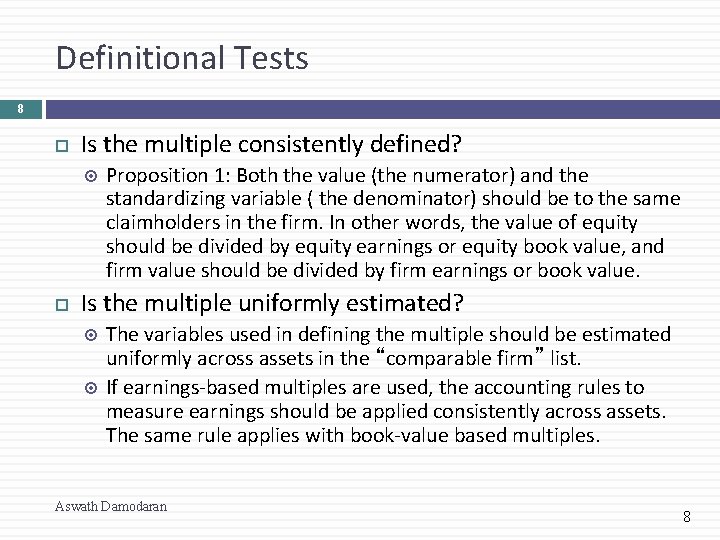
Definitional Tests 8 Is the multiple consistently defined? Proposition 1: Both the value (the numerator) and the standardizing variable ( the denominator) should be to the same claimholders in the firm. In other words, the value of equity should be divided by equity earnings or equity book value, and firm value should be divided by firm earnings or book value. Is the multiple uniformly estimated? The variables used in defining the multiple should be estimated uniformly across assets in the “comparable firm” list. If earnings-based multiples are used, the accounting rules to measure earnings should be applied consistently across assets. The same rule applies with book-value based multiples. Aswath Damodaran 8

Example 1: Price Earnings Ratio: Definition 9 PE = Market Price per Share / Earnings per Share There a number of variants on the basic PE ratio in use. They are based upon how the price and the earnings are defined. Price: EPS: Aswath Damodaran is usually the current price is sometimes the average price for the year EPS in most recent financial year EPS in trailing 12 months Forecasted earnings per share next year Forecasted earnings per share in future year 9

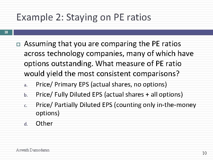
Example 2: Staying on PE ratios 10 Assuming that you are comparing the PE ratios across technology companies, many of which have options outstanding. What measure of PE ratio would yield the most consistent comparisons? a. b. c. d. Price/ Primary EPS (actual shares, no options) Price/ Fully Diluted EPS (actual shares + all options) Price/ Partially Diluted EPS (counting only in-the-money options) Other Aswath Damodaran 10

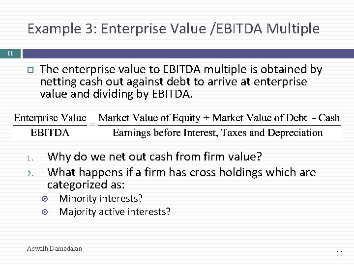
Example 3: Enterprise Value /EBITDA Multiple 11 1. 2. The enterprise value to EBITDA multiple is obtained by netting cash out against debt to arrive at enterprise value and dividing by EBITDA. Why do we net out cash from firm value? What happens if a firm has cross holdings which are categorized as: Minority interests? Majority active interests? Aswath Damodaran 11

Example 4: A Housing Price Multiple 12 The bubbles and busts in housing prices has led investors to search for a multiple that they can use to determine when housing prices are getting out of line. One measure that has acquired adherents is the ratio of housing price to annual net rental income (for renting out the same house). Assume that you decide to compute this ratio and compare it to the multiple at which stocks are trading. Which valuation ratio would be the one that corresponds to the house price/rent ratio? a. Price Earnings Ratio b. EV to Sales c. EV to EBITDA d. EV to EBIT Aswath Damodaran 12

Descriptive Tests 13 What is the average and standard deviation for this multiple, across the universe (market)? What is the median for this multiple? How large are the outliers to the distribution, and how do we deal with the outliers? The median for this multiple is often a more reliable comparison point. Throwing out the outliers may seem like an obvious solution, but if the outliers all lie on one side of the distribution (they usually are large positive numbers), this can lead to a biased estimate. Are there cases where the multiple cannot be estimated? Will ignoring these cases lead to a biased estimate of the multiple? How has this multiple changed over time? Aswath Damodaran 13

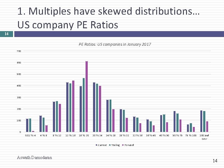
1. Multiples have skewed distributions… US company PE Ratios 14 PE Ratios: US companies in January 2017 700 600 500 400 300 200 100 0 0. 01 To 4 4 To 8 8 To 12 12 To 16 16 To 20 20 To 24 24 To 28 Current Aswath Damodaran 28 To 32 Trailing 32 To 36 36 To 40 40 To 50 50 To 75 75 To 100 and over Forward 14

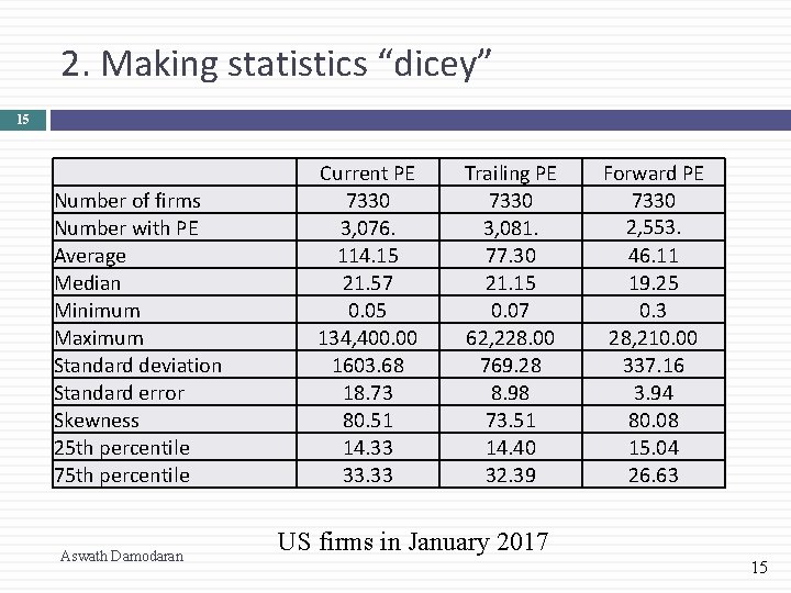
2. Making statistics “dicey” 15 Number of firms Number with PE Average Median Minimum Maximum Standard deviation Standard error Skewness 25 th percentile 75 th percentile Aswath Damodaran Current PE 7330 3, 076. 114. 15 21. 57 0. 05 134, 400. 00 1603. 68 18. 73 80. 51 14. 33 33. 33 Trailing PE 7330 3, 081. 77. 30 21. 15 0. 07 62, 228. 00 769. 28 8. 98 73. 51 14. 40 32. 39 Forward PE 7330 2, 553. 46. 11 19. 25 0. 3 28, 210. 00 337. 16 3. 94 80. 08 15. 04 26. 63 US firms in January 2017 15

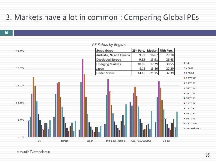
3. Markets have a lot in common : Comparing Global PEs 16 PE Ratios by Region 25. 00% <4 4 To 8 20. 00% 8 To 12 12 To 16 16 To 20 15. 00% 20 To 24 24 To 28 28 To 32 10. 00% 32 To 36 36 To 40 40 To 50 50 To 75 5. 00% 75 To 100 and over 0. 00% US Aswath Damodaran Europe Japan Emerging Markets Aus, NZ & Canada Global 16

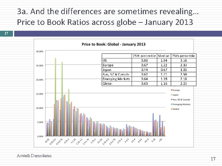
3 a. And the differences are sometimes revealing… Price to Book Ratios across globe – January 2013 17 Aswath Damodaran 17

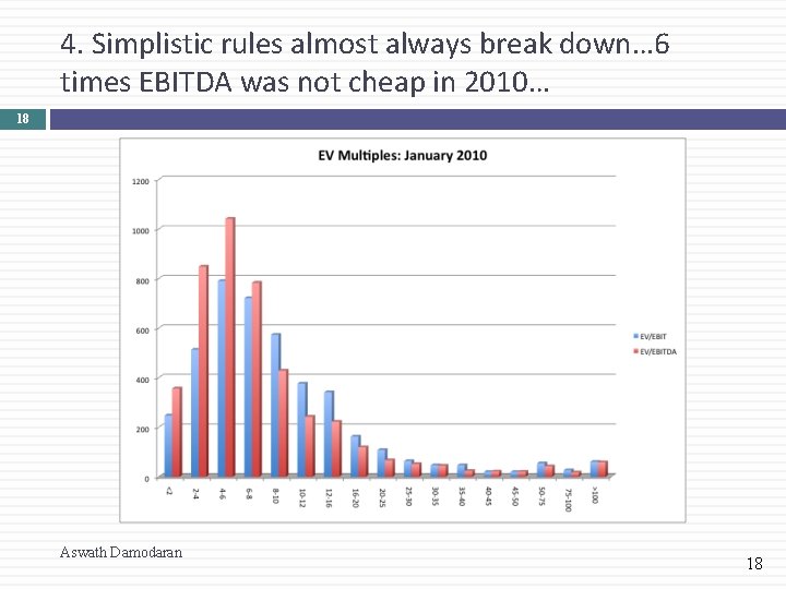
4. Simplistic rules almost always break down… 6 times EBITDA was not cheap in 2010… 18 Aswath Damodaran 18

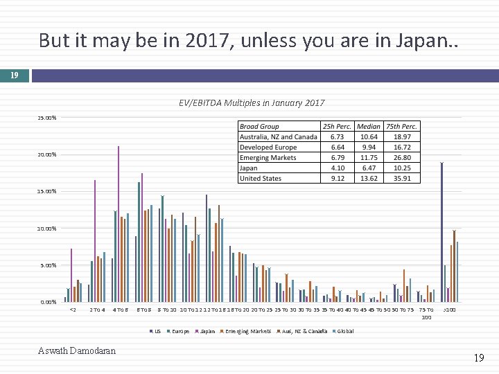
But it may be in 2017, unless you are in Japan. . 19 EV/EBITDA Multiples in January 2017 25. 00% 20. 00% 15. 00% 10. 00% 5. 00% 0. 00% <2 2 To 4 4 To 6 6 To 8 8 To 10 10 To 12 12 To 16 16 To 20 20 To 25 25 To 30 30 To 35 35 To 40 40 To 45 45 To 50 50 To 75 75 To 100 US Aswath Damodaran Europe Japan Emerging Markets Aus, NZ & Canada >100 Global 19

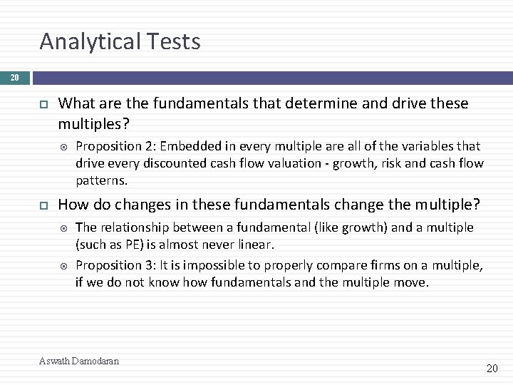
Analytical Tests 20 What are the fundamentals that determine and drive these multiples? Proposition 2: Embedded in every multiple are all of the variables that drive every discounted cash flow valuation - growth, risk and cash flow patterns. How do changes in these fundamentals change the multiple? The relationship between a fundamental (like growth) and a multiple (such as PE) is almost never linear. Proposition 3: It is impossible to properly compare firms on a multiple, if we do not know how fundamentals and the multiple move. Aswath Damodaran 20

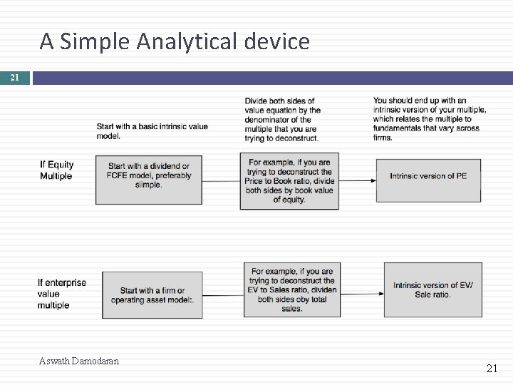
A Simple Analytical device 21 Aswath Damodaran 21

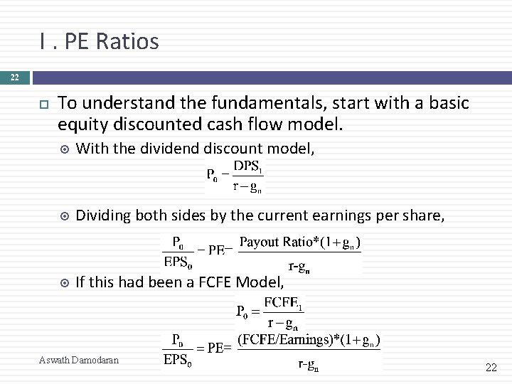
I. PE Ratios 22 To understand the fundamentals, start with a basic equity discounted cash flow model. With the dividend discount model, Dividing both sides by the current earnings per share, If this had been a FCFE Model, Aswath Damodaran 22

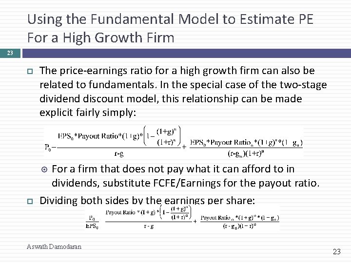
Using the Fundamental Model to Estimate PE For a High Growth Firm 23 The price-earnings ratio for a high growth firm can also be related to fundamentals. In the special case of the two-stage dividend discount model, this relationship can be made explicit fairly simply: For a firm that does not pay what it can afford to in dividends, substitute FCFE/Earnings for the payout ratio. Dividing both sides by the earnings per share: Aswath Damodaran 23

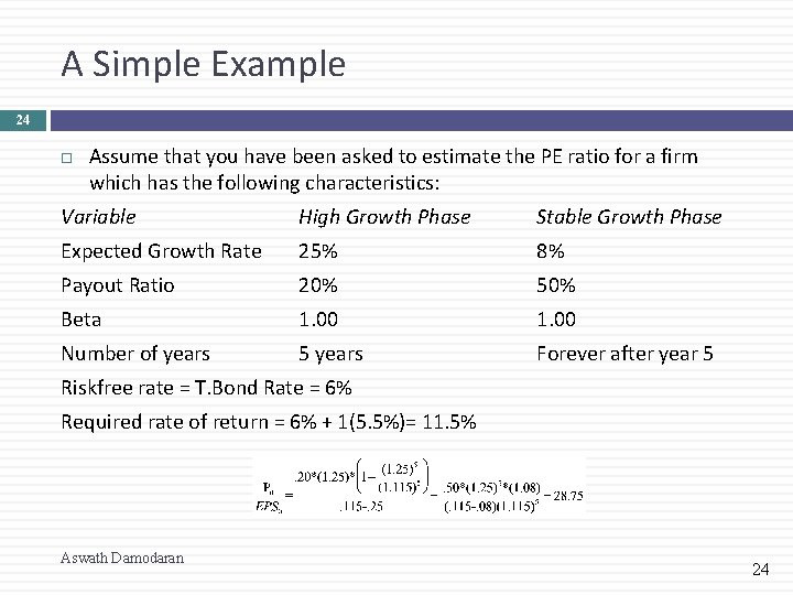
A Simple Example 24 Assume that you have been asked to estimate the PE ratio for a firm which has the following characteristics: Variable High Growth Phase Stable Growth Phase Expected Growth Rate 25% 8% Payout Ratio 20% 50% Beta 1. 00 Number of years 5 years Forever after year 5 Riskfree rate = T. Bond Rate = 6% Required rate of return = 6% + 1(5. 5%)= 11. 5% Aswath Damodaran 24

a. PE and Growth: Firm grows at x% for 5 years, 8% thereafter 25 Aswath Damodaran 25

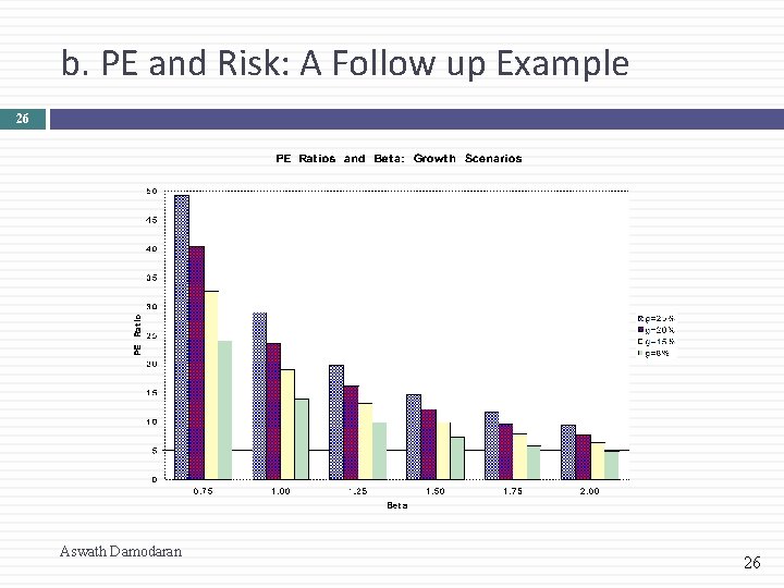
b. PE and Risk: A Follow up Example 26 Aswath Damodaran 26

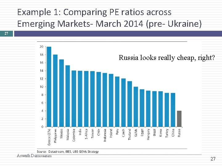
Example 1: Comparing PE ratios across Emerging Markets- March 2014 (pre- Ukraine) 27 Russia looks really cheap, right? Aswath Damodaran 27

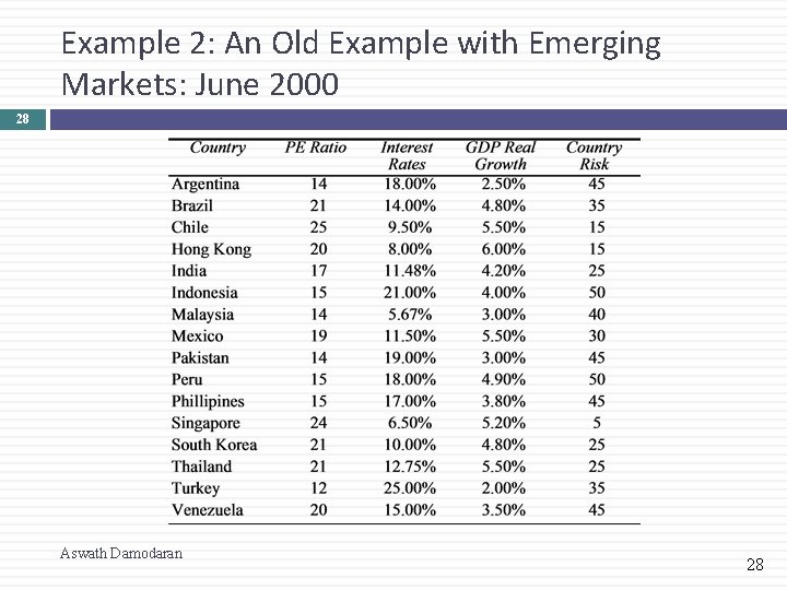
Example 2: An Old Example with Emerging Markets: June 2000 28 Aswath Damodaran 28

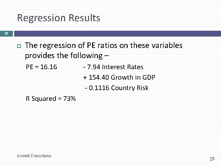
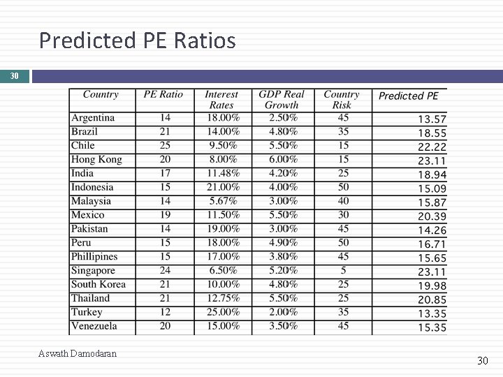
Regression Results 29 The regression of PE ratios on these variables provides the following – PE = 16. 16 - 7. 94 Interest Rates + 154. 40 Growth in GDP - 0. 1116 Country Risk R Squared = 73% Aswath Damodaran 29

Predicted PE Ratios 30 Aswath Damodaran 30

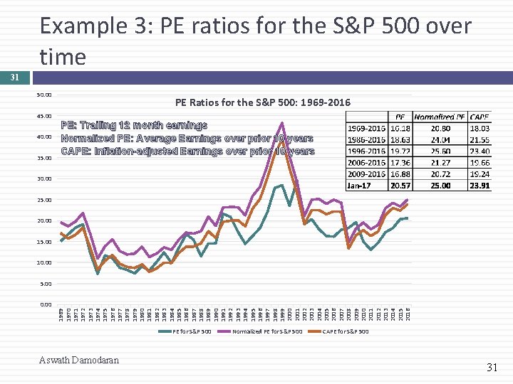
Example 3: PE ratios for the S&P 500 over time 31 50. 00 PE Ratios for the S&P 500: 1969 -2016 45. 00 40. 00 35. 00 PE: Trailing 12 month earnings Normalized PE: Average Earnings over prior 10 years CAPE: Inflation-adjusted Earnings over prior 10 years 30. 00 25. 00 20. 00 15. 00 10. 00 1969 1970 1971 1972 1973 1974 1975 1976 1977 1978 1979 1980 1981 1982 1983 1984 1985 1986 1987 1988 1989 1990 1991 1992 1993 1994 1995 1996 1997 1998 1999 2000 2001 2002 2003 2004 2005 2006 2007 2008 2009 2010 2011 2012 2013 2014 2015 2016 5. 00 PE for S&P 500 Aswath Damodaran Normalized PE for S&P 500 CAPE for S&P 500 31

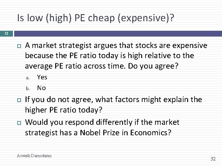
Is low (high) PE cheap (expensive)? 32 A market strategist argues that stocks are expensive because the PE ratio today is high relative to the average PE ratio across time. Do you agree? a. b. Yes No If you do not agree, what factors might explain the higher PE ratio today? Would you respond differently if the market strategist has a Nobel Prize in Economics? Aswath Damodaran 32

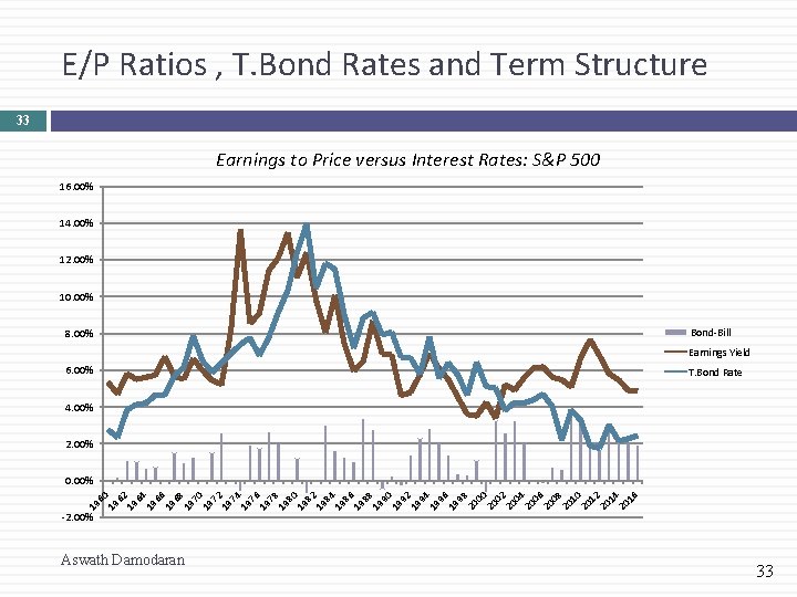
E/P Ratios , T. Bond Rates and Term Structure 33 Earnings to Price versus Interest Rates: S&P 500 16. 00% 14. 00% 12. 00% 10. 00% 8. 00% Bond-Bill Earnings Yield 6. 00% T. Bond Rate 4. 00% 2. 00% 19 60 19 62 19 64 19 66 19 68 19 70 19 72 19 74 19 76 19 78 19 80 19 82 19 84 19 86 19 88 19 90 19 92 19 94 19 96 19 98 20 00 20 02 20 04 20 06 20 08 20 10 20 12 20 14 20 16 0. 00% -2. 00% Aswath Damodaran 33

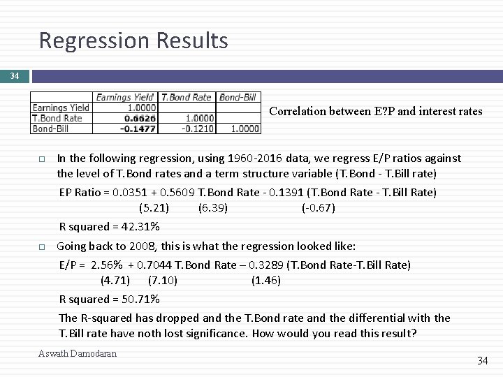
Regression Results 34 Correlation between E? P and interest rates In the following regression, using 1960 -2016 data, we regress E/P ratios against the level of T. Bond rates and a term structure variable (T. Bond - T. Bill rate) EP Ratio = 0. 0351 + 0. 5609 T. Bond Rate - 0. 1391 (T. Bond Rate - T. Bill Rate) (5. 21) (6. 39) (-0. 67) R squared = 42. 31% Going back to 2008, this is what the regression looked like: E/P = 2. 56% + 0. 7044 T. Bond Rate – 0. 3289 (T. Bond Rate-T. Bill Rate) (4. 71) (7. 10) (1. 46) R squared = 50. 71% The R-squared has dropped and the T. Bond rate and the differential with the T. Bill rate have noth lost significance. How would you read this result? Aswath Damodaran 34

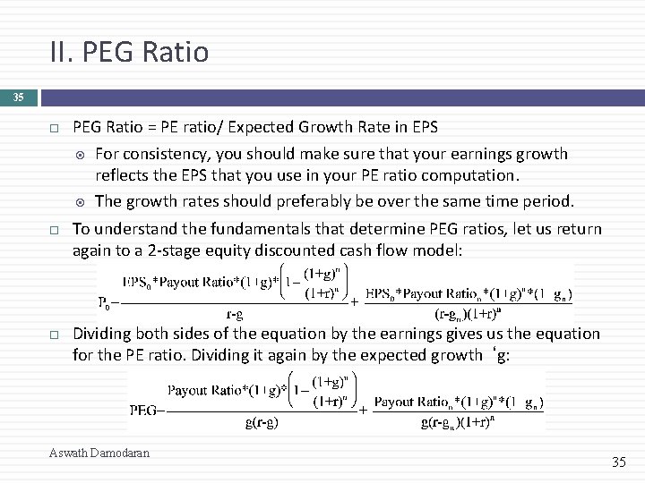
II. PEG Ratio 35 PEG Ratio = PE ratio/ Expected Growth Rate in EPS For consistency, you should make sure that your earnings growth reflects the EPS that you use in your PE ratio computation. The growth rates should preferably be over the same time period. To understand the fundamentals that determine PEG ratios, let us return again to a 2 -stage equity discounted cash flow model: Dividing both sides of the equation by the earnings gives us the equation for the PE ratio. Dividing it again by the expected growth ‘g: Aswath Damodaran 35

PEG Ratios and Fundamentals 36 Risk and payout, which affect PE ratios, continue to affect PEG ratios as well. Implication: When comparing PEG ratios across companies, we are making implicit or explicit assumptions about these variables. Dividing PE by expected growth does not neutralize the effects of expected growth, since the relationship between growth and value is not linear and fairly complex (even in a 2 -stage model) Aswath Damodaran 36

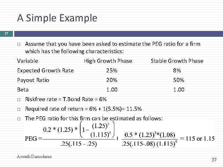
A Simple Example 37 Assume that you have been asked to estimate the PEG ratio for a firm which has the following characteristics: Variable High Growth Phase Stable Growth Phase Expected Growth Rate 25% 8% Payout Ratio 20% 50% Beta 1. 00 Riskfree rate = T. Bond Rate = 6% Required rate of return = 6% + 1(5. 5%)= 11. 5% The PEG ratio for this firm can be estimated as follows: Aswath Damodaran 37

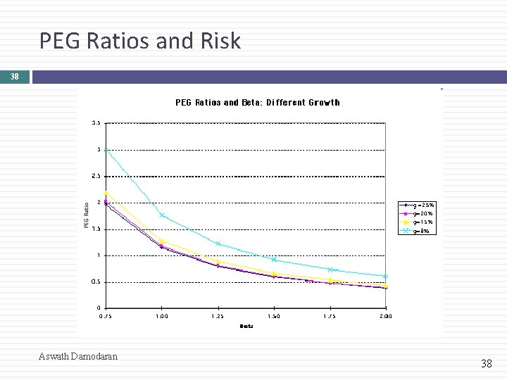
PEG Ratios and Risk 38 Aswath Damodaran 38

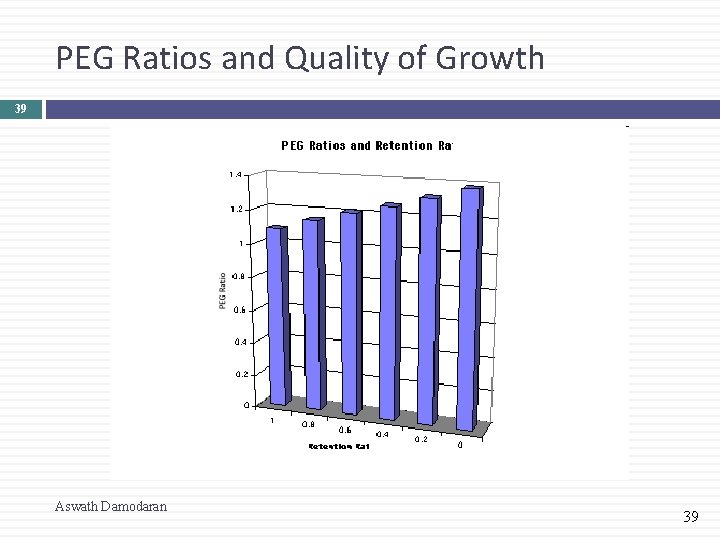
PEG Ratios and Quality of Growth 39 Aswath Damodaran 39

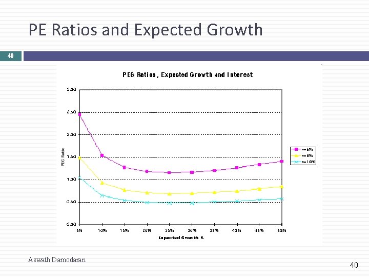
PE Ratios and Expected Growth 40 Aswath Damodaran 40

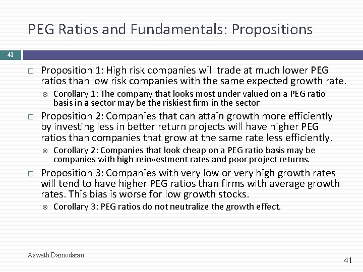
PEG Ratios and Fundamentals: Propositions 41 Proposition 1: High risk companies will trade at much lower PEG ratios than low risk companies with the same expected growth rate. Proposition 2: Companies that can attain growth more efficiently by investing less in better return projects will have higher PEG ratios than companies that grow at the same rate less efficiently. Corollary 1: The company that looks most under valued on a PEG ratio basis in a sector may be the riskiest firm in the sector Corollary 2: Companies that look cheap on a PEG ratio basis may be companies with high reinvestment rates and poor project returns. Proposition 3: Companies with very low or very high growth rates will tend to have higher PEG ratios than firms with average growth rates. This bias is worse for low growth stocks. Corollary 3: PEG ratios do not neutralize the growth effect. Aswath Damodaran 41

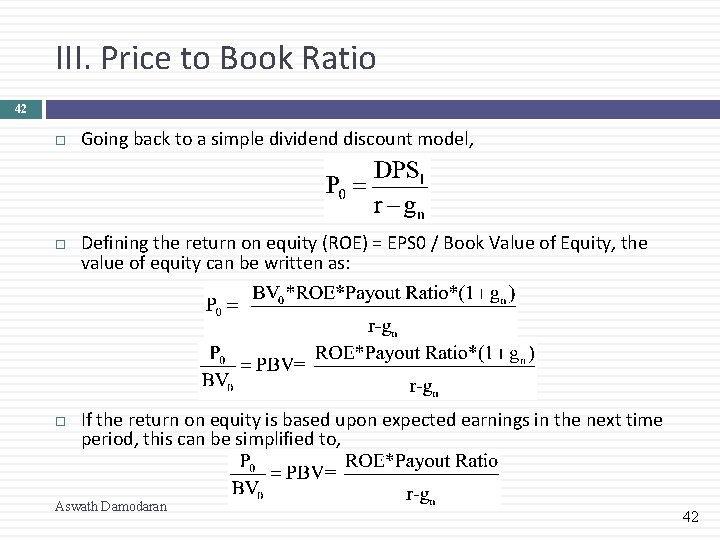
III. Price to Book Ratio 42 Going back to a simple dividend discount model, Defining the return on equity (ROE) = EPS 0 / Book Value of Equity, the value of equity can be written as: If the return on equity is based upon expected earnings in the next time period, this can be simplified to, Aswath Damodaran 42

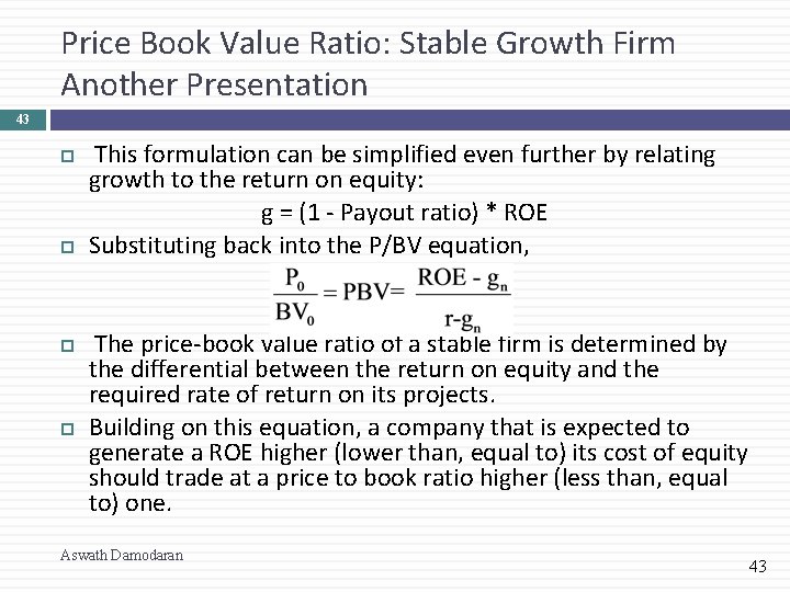
Price Book Value Ratio: Stable Growth Firm Another Presentation 43 This formulation can be simplified even further by relating growth to the return on equity: g = (1 - Payout ratio) * ROE Substituting back into the P/BV equation, The price-book value ratio of a stable firm is determined by the differential between the return on equity and the required rate of return on its projects. Building on this equation, a company that is expected to generate a ROE higher (lower than, equal to) its cost of equity should trade at a price to book ratio higher (less than, equal to) one. Aswath Damodaran 43

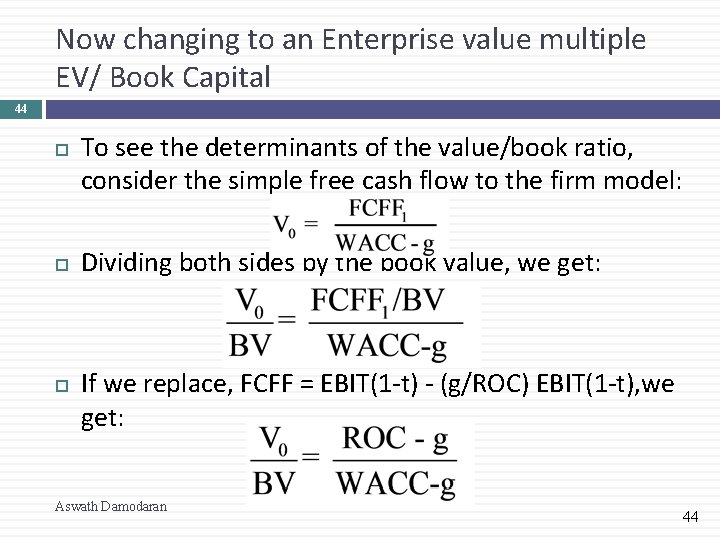
Now changing to an Enterprise value multiple EV/ Book Capital 44 To see the determinants of the value/book ratio, consider the simple free cash flow to the firm model: Dividing both sides by the book value, we get: If we replace, FCFF = EBIT(1 -t) - (g/ROC) EBIT(1 -t), we get: Aswath Damodaran 44

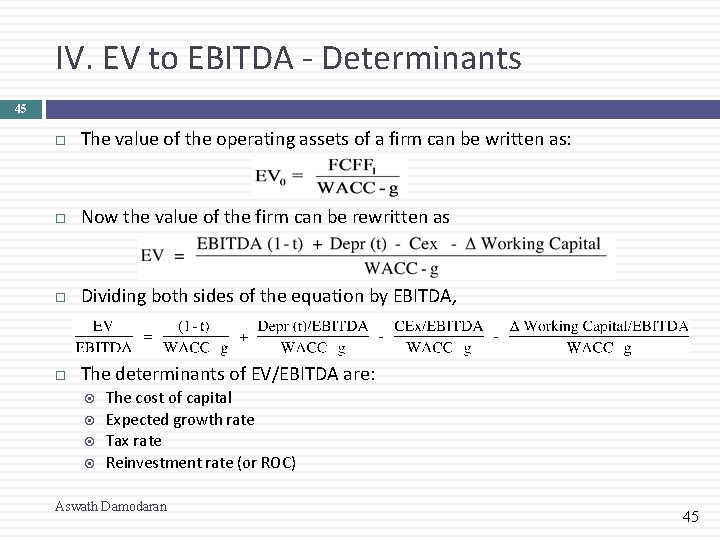
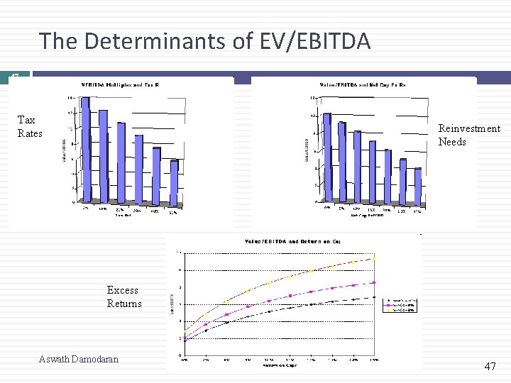
IV. EV to EBITDA - Determinants 45 The value of the operating assets of a firm can be written as: Now the value of the firm can be rewritten as Dividing both sides of the equation by EBITDA, The determinants of EV/EBITDA are: The cost of capital Expected growth rate Tax rate Reinvestment rate (or ROC) Aswath Damodaran 45

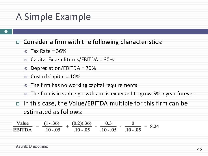
A Simple Example 46 Consider a firm with the following characteristics: Tax Rate = 36% Capital Expenditures/EBITDA = 30% Depreciation/EBITDA = 20% Cost of Capital = 10% The firm has no working capital requirements The firm is in stable growth and is expected to grow 5% a year forever. In this case, the Value/EBITDA multiple for this firm can be estimated as follows: Aswath Damodaran 46

The Determinants of EV/EBITDA 47 Tax Rates Reinvestment Needs Excess Returns Aswath Damodaran 47

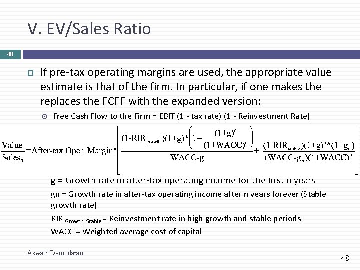
V. EV/Sales Ratio 48 If pre-tax operating margins are used, the appropriate value estimate is that of the firm. In particular, if one makes the replaces the FCFF with the expanded version: Free Cash Flow to the Firm = EBIT (1 - tax rate) (1 - Reinvestment Rate) Then the Value of the Firm can be written as a function of the after-tax operating margin= (EBIT (1 -t)/Sales g = Growth rate in after-tax operating income for the first n years gn = Growth rate in after-tax operating income after n years forever (Stable growth rate) RIR Growth, Stable = Reinvestment rate in high growth and stable periods WACC = Weighted average cost of capital Aswath Damodaran 48

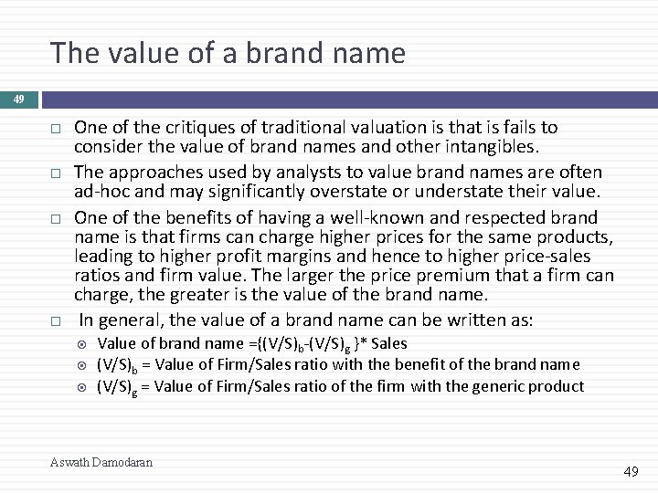
The value of a brand name 49 One of the critiques of traditional valuation is that is fails to consider the value of brand names and other intangibles. The approaches used by analysts to value brand names are often ad-hoc and may significantly overstate or understate their value. One of the benefits of having a well-known and respected brand name is that firms can charge higher prices for the same products, leading to higher profit margins and hence to higher price-sales ratios and firm value. The larger the price premium that a firm can charge, the greater is the value of the brand name. In general, the value of a brand name can be written as: Value of brand name ={(V/S)b-(V/S)g }* Sales (V/S)b = Value of Firm/Sales ratio with the benefit of the brand name (V/S)g = Value of Firm/Sales ratio of the firm with the generic product Aswath Damodaran 49

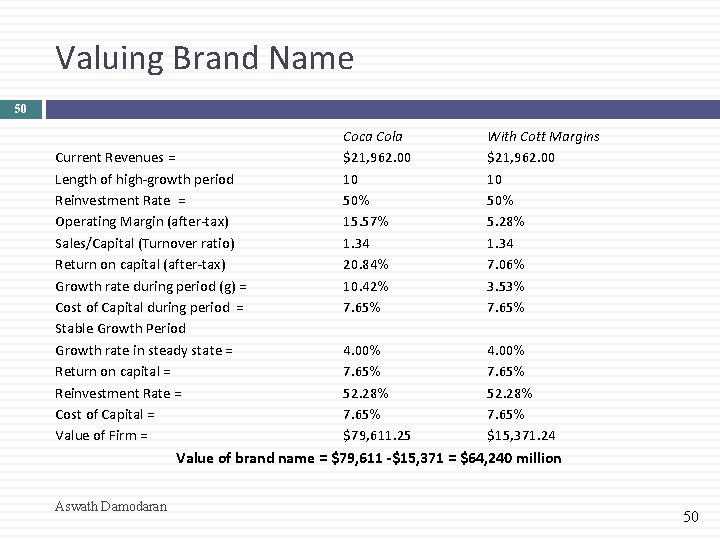
Valuing Brand Name 50 Current Revenues = Length of high-growth period Reinvestment Rate = Operating Margin (after-tax) Sales/Capital (Turnover ratio) Return on capital (after-tax) Growth rate during period (g) = Cost of Capital during period = Stable Growth Period Growth rate in steady state = Return on capital = Reinvestment Rate = Cost of Capital = Value of Firm = Coca Cola $21, 962. 00 10 50% 15. 57% 1. 34 20. 84% 10. 42% 7. 65% With Cott Margins $21, 962. 00 10 50% 5. 28% 1. 34 7. 06% 3. 53% 7. 65% 4. 00% 7. 65% 52. 28% 7. 65% $79, 611. 25 4. 00% 7. 65% 52. 28% 7. 65% $15, 371. 24 Value of brand name = $79, 611 -$15, 371 = $64, 240 million Aswath Damodaran 50

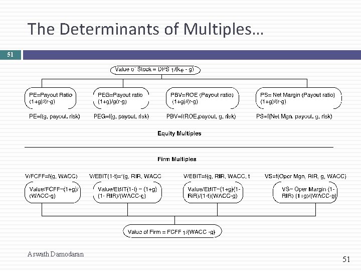
The Determinants of Multiples… 51 Aswath Damodaran 51

Application Tests 52 Given the firm that we are valuing, what is a “comparable” firm? While traditional analysis is built on the premise that firms in the same sector are comparable firms, valuation theory would suggest that a comparable firm is one which is similar to the one being analyzed in terms of fundamentals. There is no reason why a firm cannot be compared with another firm in a very different business, if the two firms have the same risk, growth and cash flow characteristics. Given the comparable firms, how do we adjust for differences across firms on the fundamentals? It is impossible to find an exactly identical firm to the one you are valuing. You need to control for differences across firms. Aswath Damodaran 52

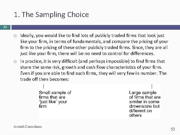
1. The Sampling Choice 53 Ideally, you would like to find lots of publicly traded firms that look just like your firm, in terms of fundamentals, and compare the pricing of your firm to the pricing of these other publicly traded firms. Since, they are all just like your firm, there will be no need to control for differences. In practice, it is very difficult (and perhaps impossible) to find firms that share the same risk, growth and cash flow characteristics of your firm. Even if you are able to find such firms, they will very few in number. The trade off then becomes: Aswath Damodaran 53

2. The ”Control for Differences” Choices 54 1. 2. Direct comparisons: If the comparable firms are “just like” your firm, you can compare multiples directly across the firms and conclude that your firm is expensive (cheap) if it trades at a multiple higher (lower) than the other firms. Story telling: If there is a key dimension on which the firms vary, you can tell a story based upon your understanding of how value varies on that dimension. An example: This company trades at 12 times earnings, whereas the rest of the sector trades at 10 times earnings, but I think it is cheap because it has a much higher growth rate than the rest of the sector. 3. 4. Modified multiple: You can modify the multiple to incorporate the dimension on which there are differences across firms. Statistical techniques: If your firms vary on more than one dimension, you can try using multiple regressions (or variants thereof) to arrive at a “controlled” estimate for your firm. Aswath Damodaran 54

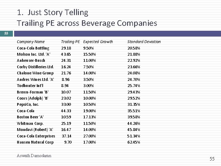
1. Just Story Telling Trailing PE across Beverage Companies 55 Company Name Trailing PE Coca-Cola Bottling 29. 18 Molson Inc. Ltd. 'A' 43. 65 Anheuser-Busch 24. 31 Corby Distilleries Ltd. 16. 24 Chalone Wine Group 21. 76 Andres Wines Ltd. 'A' 8. 96 Todhunter Int'l 8. 94 Brown-Forman 'B' 10. 07 Coors (Adolph) 'B' 23. 02 Pepsi. Co, Inc. 33. 00 Coca-Cola 44. 33 Boston Beer 'A' 10. 59 Whitman Corp. 25. 19 Mondavi (Robert) 'A' 16. 47 Coca-Cola Enterprises 37. 14 Hansen Natural Corp 9. 70 Aswath Damodaran Expected Growth 9. 50% 15. 50% 11. 00% 7. 50% 14. 00% 3. 50% 3. 00% 11. 50% 10. 00% 10. 50% 19. 00% 17. 13% 11. 50% 14. 00% 27. 00% 17. 00% Standard Deviation 20. 58% 21. 88% 22. 92% 23. 66% 24. 08% 24. 70% 25. 74% 29. 43% 29. 52% 31. 35% 35. 51% 39. 58% 44. 26% 45. 84% 51. 34% 62. 45% 55

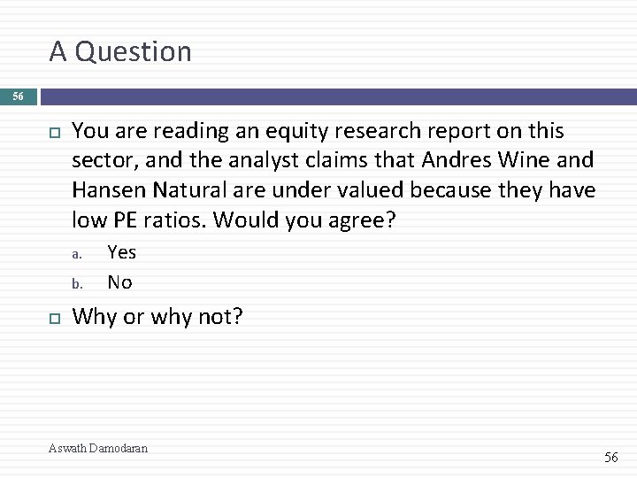
A Question 56 You are reading an equity research report on this sector, and the analyst claims that Andres Wine and Hansen Natural are under valued because they have low PE ratios. Would you agree? a. b. Yes No Why or why not? Aswath Damodaran 56

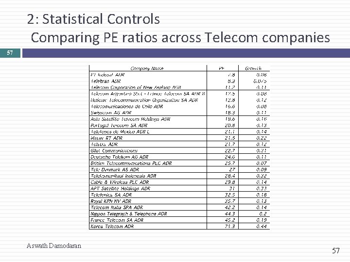
2: Statistical Controls Comparing PE ratios across Telecom companies 57 Aswath Damodaran 57

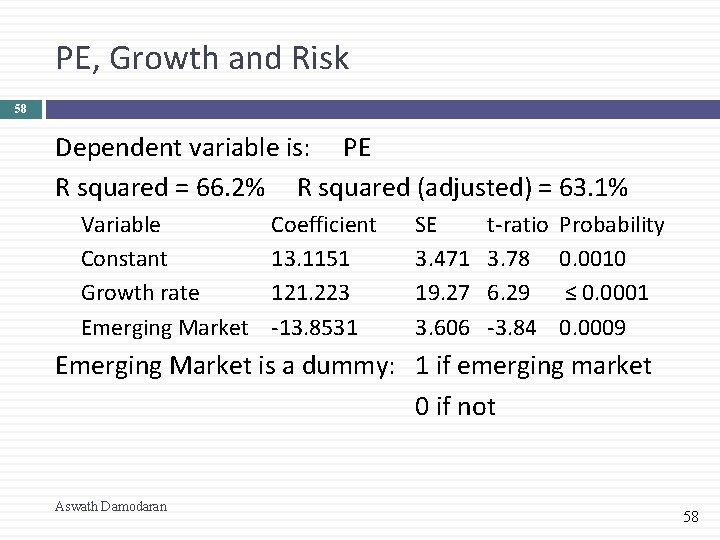
PE, Growth and Risk 58 Dependent variable is: PE R squared = 66. 2% R squared (adjusted) = 63. 1% Variable Constant Growth rate Emerging Market Coefficient 13. 1151 121. 223 -13. 8531 SE 3. 471 19. 27 3. 606 t-ratio 3. 78 6. 29 -3. 84 Probability 0. 0010 ≤ 0. 0001 0. 0009 Emerging Market is a dummy: 1 if emerging market 0 if not Aswath Damodaran 58

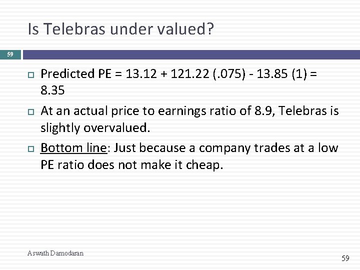
Is Telebras under valued? 59 Predicted PE = 13. 12 + 121. 22 (. 075) - 13. 85 (1) = 8. 35 At an actual price to earnings ratio of 8. 9, Telebras is slightly overvalued. Bottom line: Just because a company trades at a low PE ratio does not make it cheap. Aswath Damodaran 59

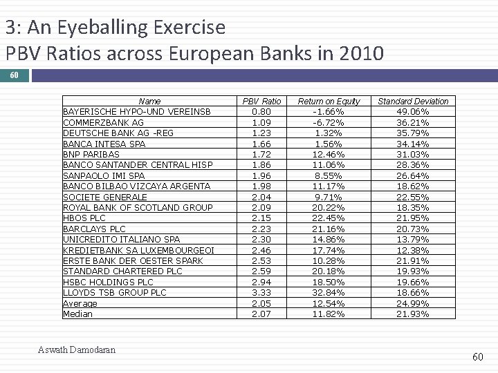
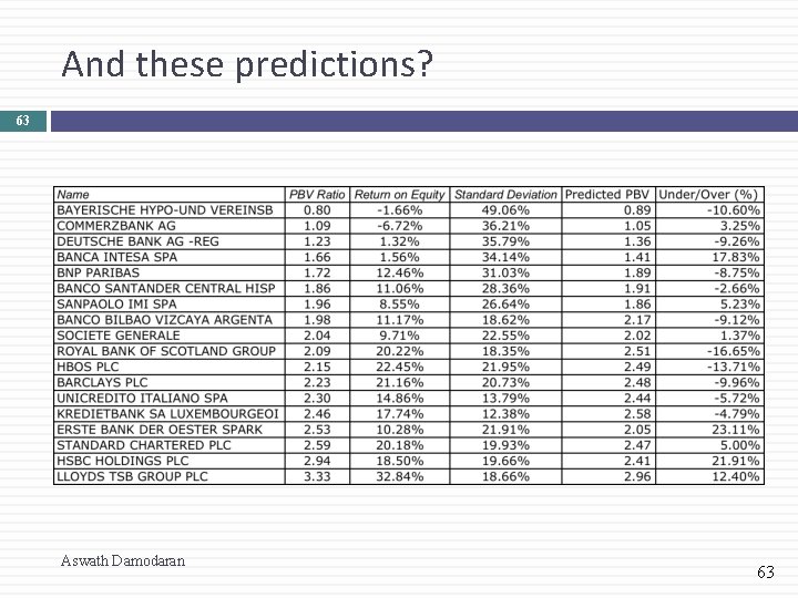
3: An Eyeballing Exercise PBV Ratios across European Banks in 2010 60 Name BAYERISCHE HYPO-UND VEREINSB COMMERZBANK AG DEUTSCHE BANK AG -REG BANCA INTESA SPA BNP PARIBAS BANCO SANTANDER CENTRAL HISP SANPAOLO IMI SPA BANCO BILBAO VIZCAYA ARGENTA SOCIETE GENERALE ROYAL BANK OF SCOTLAND GROUP HBOS PLC BARCLAYS PLC UNICREDITO ITALIANO SPA KREDIETBANK SA LUXEMBOURGEOI ERSTE BANK DER OESTER SPARK STANDARD CHARTERED PLC HSBC HOLDINGS PLC LLOYDS TSB GROUP PLC Average Median Aswath Damodaran PBV Ratio 0. 80 1. 09 1. 23 1. 66 1. 72 1. 86 1. 98 2. 04 2. 09 2. 15 2. 23 2. 30 2. 46 2. 53 2. 59 2. 94 3. 33 2. 05 2. 07 Return on Equity -1. 66% -6. 72% 1. 32% 1. 56% 12. 46% 11. 06% 8. 55% 11. 17% 9. 71% 20. 22% 22. 45% 21. 16% 14. 86% 17. 74% 10. 28% 20. 18% 18. 50% 32. 84% 12. 54% 11. 82% Standard Deviation 49. 06% 36. 21% 35. 79% 34. 14% 31. 03% 28. 36% 26. 64% 18. 62% 22. 55% 18. 35% 21. 95% 20. 73% 13. 79% 12. 38% 21. 91% 19. 93% 19. 66% 18. 66% 24. 99% 21. 93% 60

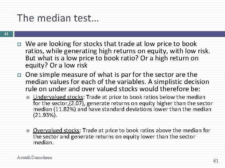
The median test… 61 We are looking for stocks that trade at low price to book ratios, while generating high returns on equity, with low risk. But what is a low price to book ratio? Or a high return on equity? Or a low risk One simple measure of what is par for the sector are the median values for each of the variables. A simplistic decision rule on under and over valued stocks would therefore be: Undervalued stocks: Trade at price to book ratios below the median for the sector, (2. 07), generate returns on equity higher than the sector median (11. 82%) and have standard deviations lower than the median (21. 93%). Overvalued stocks: Trade at price to book ratios above the median for the sector and generate returns on equity lower than the sector median. Aswath Damodaran 61

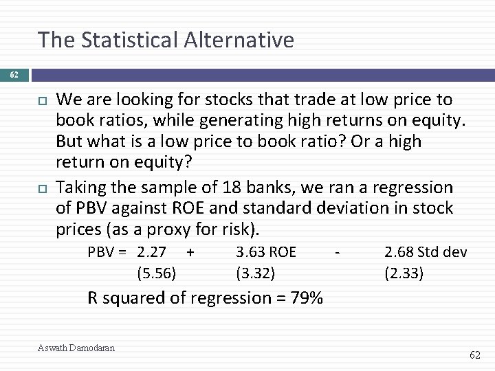
The Statistical Alternative 62 We are looking for stocks that trade at low price to book ratios, while generating high returns on equity. But what is a low price to book ratio? Or a high return on equity? Taking the sample of 18 banks, we ran a regression of PBV against ROE and standard deviation in stock prices (as a proxy for risk). PBV = 2. 27 + (5. 56) 3. 63 ROE (3. 32) - 2. 68 Std dev (2. 33) R squared of regression = 79% Aswath Damodaran 62

And these predictions? 63 Aswath Damodaran 63

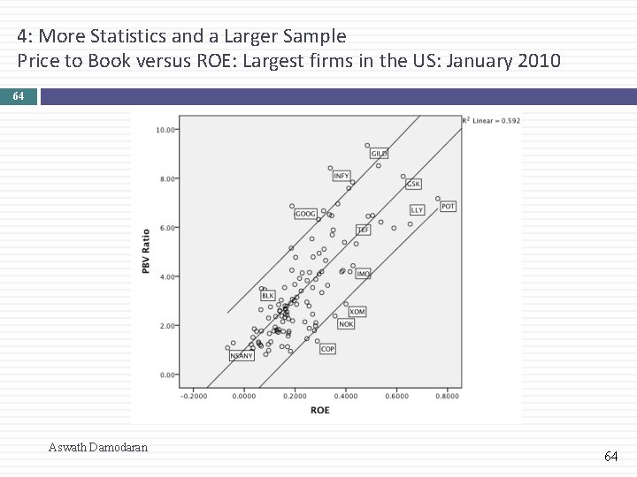
4: More Statistics and a Larger Sample Price to Book versus ROE: Largest firms in the US: January 2010 64 Aswath Damodaran 64

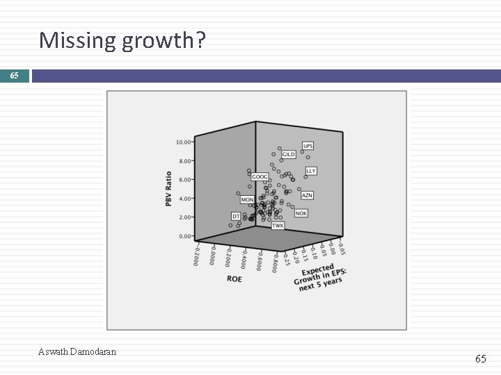
Missing growth? 65 Aswath Damodaran 65

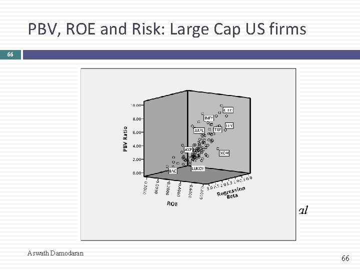
PBV, ROE and Risk: Large Cap US firms 66 Most overval ued Cheapest Most underval ued Aswath Damodaran 66

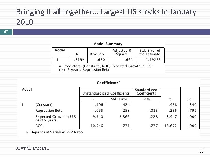
Bringing it all together… Largest US stocks in January 2010 67 Aswath Damodaran 67

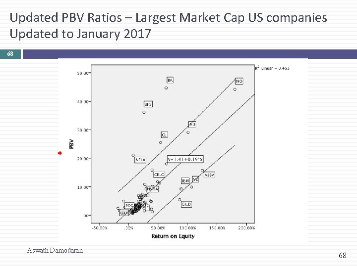
Updated PBV Ratios – Largest Market Cap US companies Updated to January 2017 68 Aswath Damodaran 68

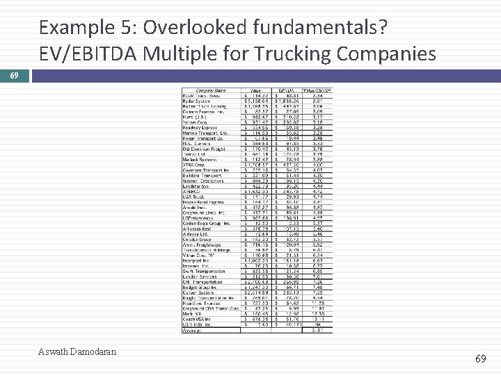
Example 5: Overlooked fundamentals? EV/EBITDA Multiple for Trucking Companies 69 Aswath Damodaran 69

A Test on EBITDA 70 Ryder System looks very cheap on a Value/EBITDA multiple basis, relative to the rest of the sector. What explanation (other than misvaluation) might there be for this difference? What general lessons would you draw from this on the EV/EBITDA multiples for infrastructure companies as their infrastructure ages? Aswath Damodaran 70

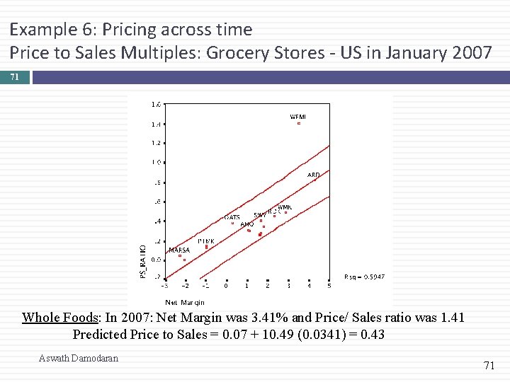
Example 6: Pricing across time Price to Sales Multiples: Grocery Stores - US in January 2007 71 Whole Foods: In 2007: Net Margin was 3. 41% and Price/ Sales ratio was 1. 41 Predicted Price to Sales = 0. 07 + 10. 49 (0. 0341) = 0. 43 Aswath Damodaran 71

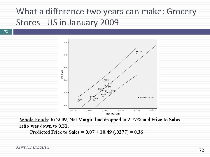
What a difference two years can make: Grocery Stores - US in January 2009 72 Whole Foods: In 2009, Net Margin had dropped to 2. 77% and Price to Sales ratio was down to 0. 31. Predicted Price to Sales = 0. 07 + 10. 49 (. 0277) = 0. 36 Aswath Damodaran 72

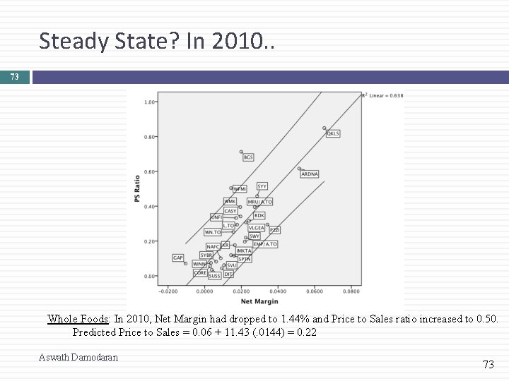
Steady State? In 2010. . 73 Whole Foods: In 2010, Net Margin had dropped to 1. 44% and Price to Sales ratio increased to 0. 50. Predicted Price to Sales = 0. 06 + 11. 43 (. 0144) = 0. 22 Aswath Damodaran 73

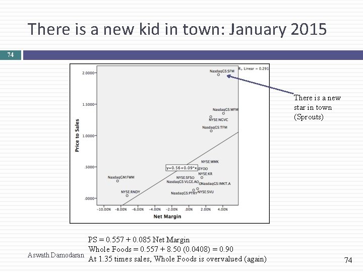
There is a new kid in town: January 2015 74 There is a new star in town (Sprouts) PS = 0. 557 + 0. 085 Net Margin Whole Foods = 0. 557 + 8. 50 (0. 0408) = 0. 90 Aswath Damodaran At 1. 35 times sales, Whole Foods is overvalued (again) 74

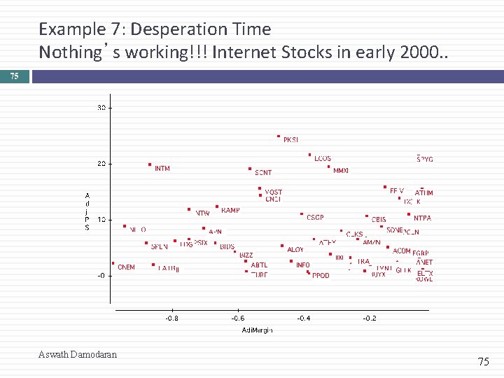
Example 7: Desperation Time Nothing’s working!!! Internet Stocks in early 2000. . 75 Aswath Damodaran 75

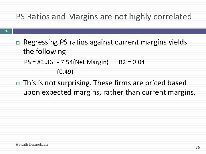
PS Ratios and Margins are not highly correlated 76 Regressing PS ratios against current margins yields the following PS = 81. 36 - 7. 54(Net Margin) (0. 49) R 2 = 0. 04 This is not surprising. These firms are priced based upon expected margins, rather than current margins. Aswath Damodaran 76

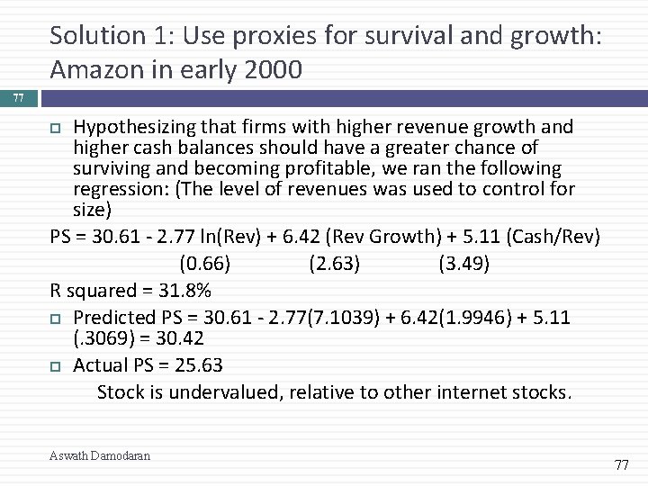
Solution 1: Use proxies for survival and growth: Amazon in early 2000 77 Hypothesizing that firms with higher revenue growth and higher cash balances should have a greater chance of surviving and becoming profitable, we ran the following regression: (The level of revenues was used to control for size) PS = 30. 61 - 2. 77 ln(Rev) + 6. 42 (Rev Growth) + 5. 11 (Cash/Rev) (0. 66) (2. 63) (3. 49) R squared = 31. 8% Predicted PS = 30. 61 - 2. 77(7. 1039) + 6. 42(1. 9946) + 5. 11 (. 3069) = 30. 42 Actual PS = 25. 63 Stock is undervalued, relative to other internet stocks. Aswath Damodaran 77

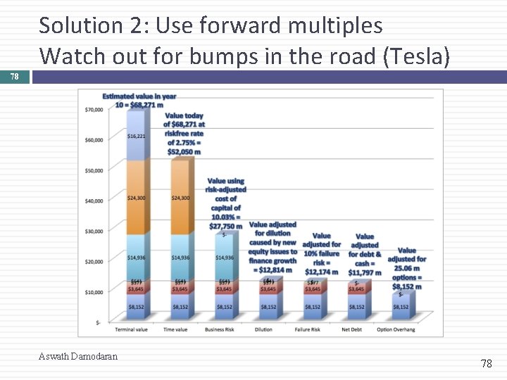
Solution 2: Use forward multiples Watch out for bumps in the road (Tesla) 78 Aswath Damodaran 78

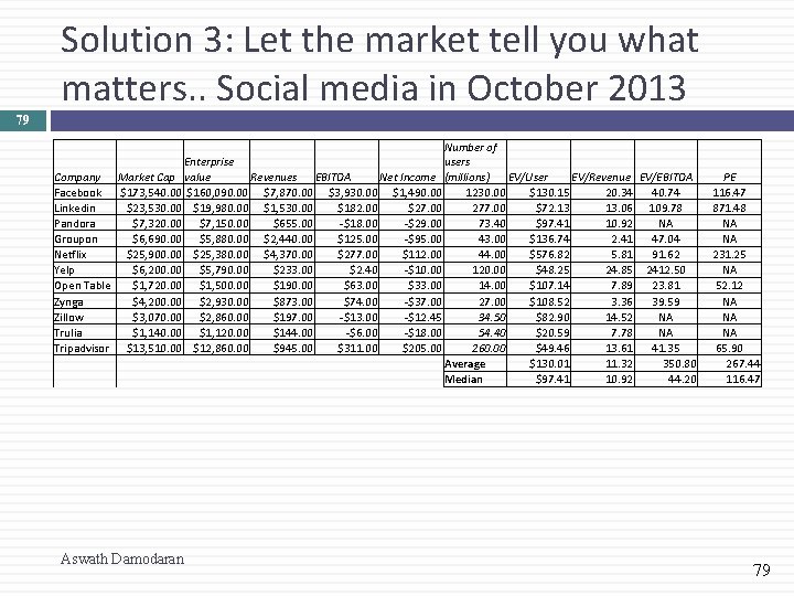
Solution 3: Let the market tell you what matters. . Social media in October 2013 79 Number of users Enterprise Company Market Cap value Revenues EBITDA Net Income (millions) EV/User EV/Revenue EV/EBITDA Facebook $173, 540. 00 $160, 090. 00 $7, 870. 00 $3, 930. 00 $1, 490. 00 1230. 00 $130. 15 20. 34 40. 74 Linkedin $23, 530. 00 $19, 980. 00 $1, 530. 00 $182. 00 $27. 00 277. 00 $72. 13 13. 06 109. 78 Pandora $7, 320. 00 $7, 150. 00 $655. 00 -$18. 00 -$29. 00 73. 40 $97. 41 10. 92 NA Groupon $6, 690. 00 $5, 880. 00 $2, 440. 00 $125. 00 -$95. 00 43. 00 $136. 74 2. 41 47. 04 Netflix $25, 900. 00 $25, 380. 00 $4, 370. 00 $277. 00 $112. 00 44. 00 $576. 82 5. 81 91. 62 Yelp $6, 200. 00 $5, 790. 00 $233. 00 $2. 40 -$10. 00 120. 00 $48. 25 24. 85 2412. 50 Open Table $1, 720. 00 $1, 500. 00 $190. 00 $63. 00 $33. 00 14. 00 $107. 14 7. 89 23. 81 Zynga $4, 200. 00 $2, 930. 00 $873. 00 $74. 00 -$37. 00 27. 00 $108. 52 3. 36 39. 59 Zillow $3, 070. 00 $2, 860. 00 $197. 00 -$13. 00 -$12. 45 34. 50 $82. 90 14. 52 NA Trulia $1, 140. 00 $1, 120. 00 $144. 00 -$6. 00 -$18. 00 54. 40 $20. 59 7. 78 NA Tripadvisor $13, 510. 00 $12, 860. 00 $945. 00 $311. 00 $205. 00 260. 00 $49. 46 13. 61 41. 35 Average $130. 01 11. 32 350. 80 Median $97. 41 10. 92 44. 20 Aswath Damodaran PE 116. 47 871. 48 NA NA 231. 25 NA 52. 12 NA NA NA 65. 90 267. 44 116. 47 79

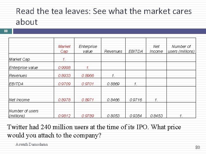
Read the tea leaves: See what the market cares about 80 Market Cap Enterprise value EBITDA Net Income Number of users (millions) Revenues 1. Enterprise value 0. 9998 1. Revenues 0. 8933 0. 8966 1. EBITDA 0. 9709 0. 9701 0. 8869 1. Net Income 0. 8978 0. 8971 0. 8466 0. 9716 1. Number of users (millions) 0. 9812 0. 9789 0. 8053 0. 9354 0. 8453 1. Market Cap Twitter had 240 million users at the time of its IPO. What price would you attach to the company? Aswath Damodaran 80

Pricing across the entire market: Why not? 81 In contrast to the 'comparable firm' approach, the information in the entire cross-section of firms can be used to predict PE ratios. The simplest way of summarizing this information is with a multiple regression, with the PE ratio as the dependent variable, and proxies for risk, growth and payout forming the independent variables. Aswath Damodaran 81

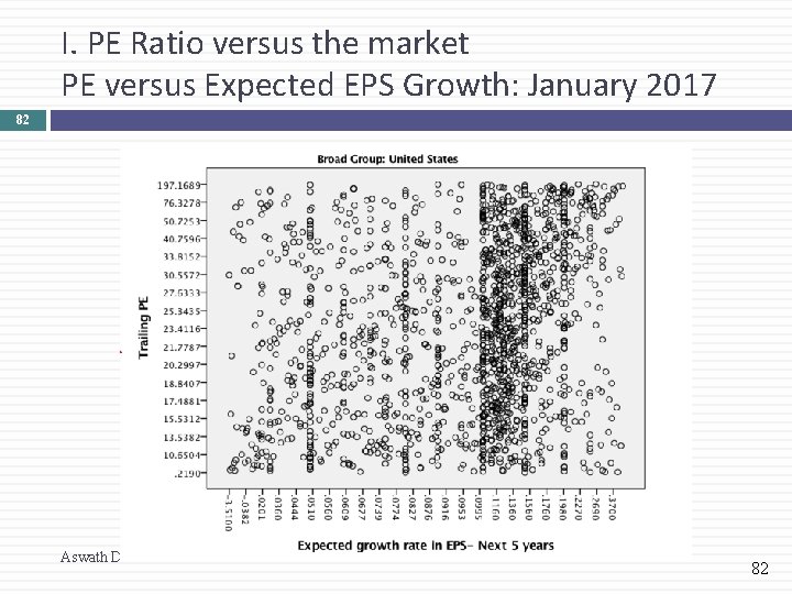
I. PE Ratio versus the market PE versus Expected EPS Growth: January 2017 82 Aswath Damodaran 82

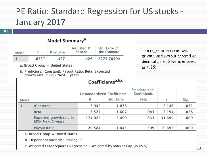
PE Ratio: Standard Regression for US stocks - January 2017 83 The regression is run with growth and payout entered as decimals, i. e. , 25% is entered as 0. 25) Aswath Damodaran 83

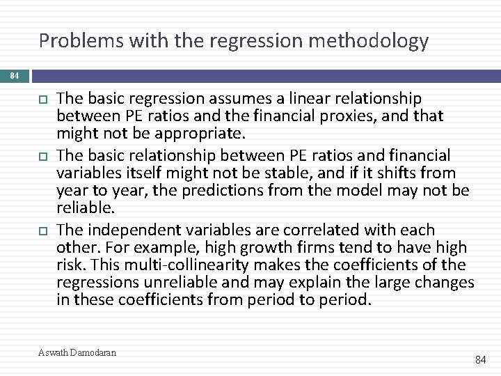
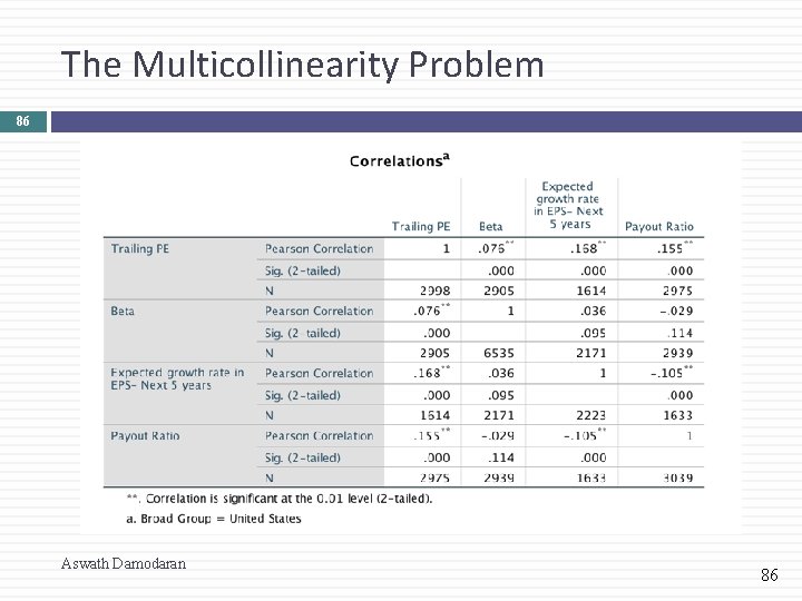
Problems with the regression methodology 84 The basic regression assumes a linear relationship between PE ratios and the financial proxies, and that might not be appropriate. The basic relationship between PE ratios and financial variables itself might not be stable, and if it shifts from year to year, the predictions from the model may not be reliable. The independent variables are correlated with each other. For example, high growth firms tend to have high risk. This multi-collinearity makes the coefficients of the regressions unreliable and may explain the large changes in these coefficients from period to period. Aswath Damodaran 84

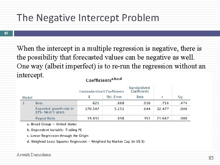
The Negative Intercept Problem 85 When the intercept in a multiple regression is negative, there is the possibility that forecasted values can be negative as well. One way (albeit imperfect) is to re-run the regression without an intercept. Aswath Damodaran 85

The Multicollinearity Problem 86 Aswath Damodaran 86

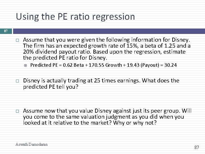
Using the PE ratio regression 87 Assume that you were given the following information for Disney. The firm has an expected growth rate of 15%, a beta of 1. 25 and a 20% dividend payout ratio. Based upon the regression, estimate the predicted PE ratio for Disney. Predicted PE = 0. 62 Beta + 170. 55 Growth + 19. 43 (Payout) = 30. 24 Disney is actually trading at 25 times earnings. What does the predicted PE tell you? Assume now that you value Disney against just its peer group. Will you come to the same valuation judgment as you did when you looked at it relative to the market? Why or why not? Aswath Damodaran 87

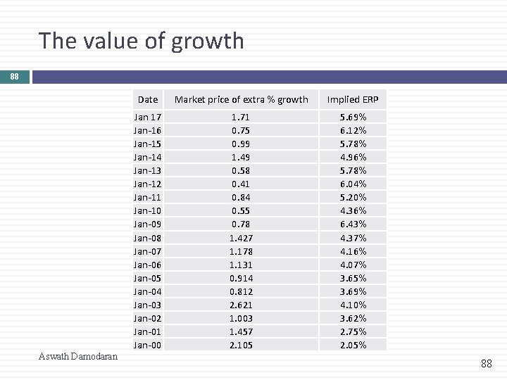
The value of growth 88 Aswath Damodaran Date Market price of extra % growth Implied ERP Jan 17 Jan-16 Jan-15 Jan-14 Jan-13 Jan-12 Jan-11 Jan-10 Jan-09 Jan-08 Jan-07 Jan-06 Jan-05 Jan-04 Jan-03 Jan-02 Jan-01 Jan-00 1. 71 0. 75 0. 99 1. 49 0. 58 0. 41 0. 84 0. 55 0. 78 1. 427 1. 178 1. 131 0. 914 0. 812 2. 621 1. 003 1. 457 2. 105 5. 69% 6. 12% 5. 78% 4. 96% 5. 78% 6. 04% 5. 20% 4. 36% 6. 43% 4. 37% 4. 16% 4. 07% 3. 65% 3. 69% 4. 10% 3. 62% 2. 75% 2. 05% 88

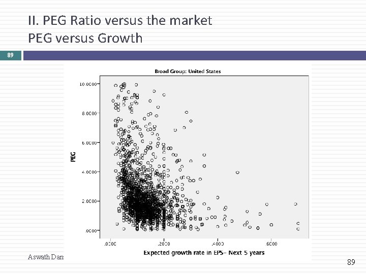
II. PEG Ratio versus the market PEG versus Growth 89 Aswath Damodaran 89

PEG versus ln(Expected Growth) 90 Aswath Damodaran 90

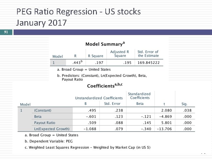
PEG Ratio Regression - US stocks January 2017 91 Aswath Damodaran 91

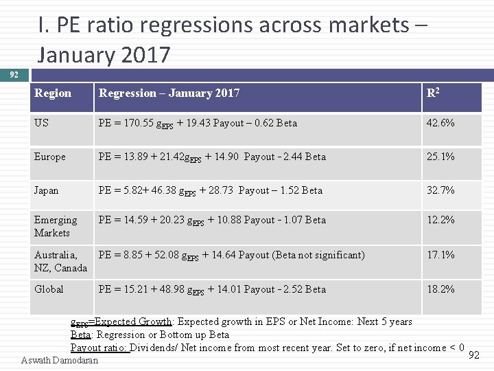
I. PE ratio regressions across markets – January 2017 92 Region Regression – January 2017 R 2 US PE = 170. 55 g. EPS + 19. 43 Payout – 0. 62 Beta 42. 6% Europe PE = 13. 89 + 21. 42 g. EPS + 14. 90 Payout – 2. 44 Beta 25. 1% Japan PE = 5. 82+ 46. 38 g. EPS + 28. 73 Payout – 1. 52 Beta 32. 7% Emerging Markets PE = 14. 59 + 20. 23 g. EPS + 10. 88 Payout – 1. 07 Beta 12. 2% Australia, NZ, Canada PE = 8. 85 + 52. 08 g. EPS + 14. 64 Payout (Beta not significant) 17. 1% Global PE = 15. 21 + 48. 98 g. EPS + 14. 01 Payout – 2. 52 Beta 18. 2% g. EPS=Expected Growth: Expected growth in EPS or Net Income: Next 5 years Beta: Regression or Bottom up Beta Payout ratio: Dividends/ Net income from most recent year. Set to zero, if net income < 0 Aswath Damodaran 92

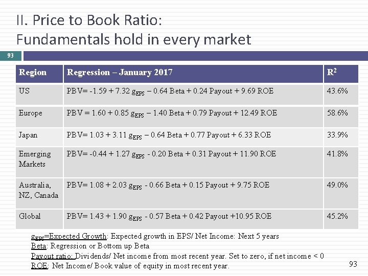
II. Price to Book Ratio: Fundamentals hold in every market 93 Region Regression – January 2017 R 2 US PBV= -1. 59 + 7. 32 g. EPS – 0. 64 Beta + 0. 24 Payout + 9. 69 ROE 43. 6% Europe PBV = 1. 60 + 0. 85 g. EPS – 1. 40 Beta + 0. 79 Payout + 12. 49 ROE 58. 6% Japan PBV= 1. 03 + 3. 11 g. EPS – 0. 64 Beta + 0. 77 Payout + 6. 33 ROE 33. 9% Emerging Markets PBV= -0. 44 + 1. 27 g. EPS - 0. 20 Beta + 0. 31 Payout + 11. 90 ROE 41. 8% Australia, NZ, Canada PBV= 1. 08 + 2. 03 g. EPS - 0. 66 Beta + 0. 15 Payout + 9. 75 ROE 49. 0% Global PBV= 1. 43 + 1. 90 g. EPS - 0. 57 Beta + 0. 42 Payout +10. 95 ROE 45. 2% g. EPS=Expected Growth: Expected growth in EPS/ Net Income: Next 5 years Beta: Regression or Bottom up Beta Payout ratio: Dividends/ Net income from most recent year. Set to zero, if net income < 0 ROE: Net Income/ Book value of equity in most recent year. 93

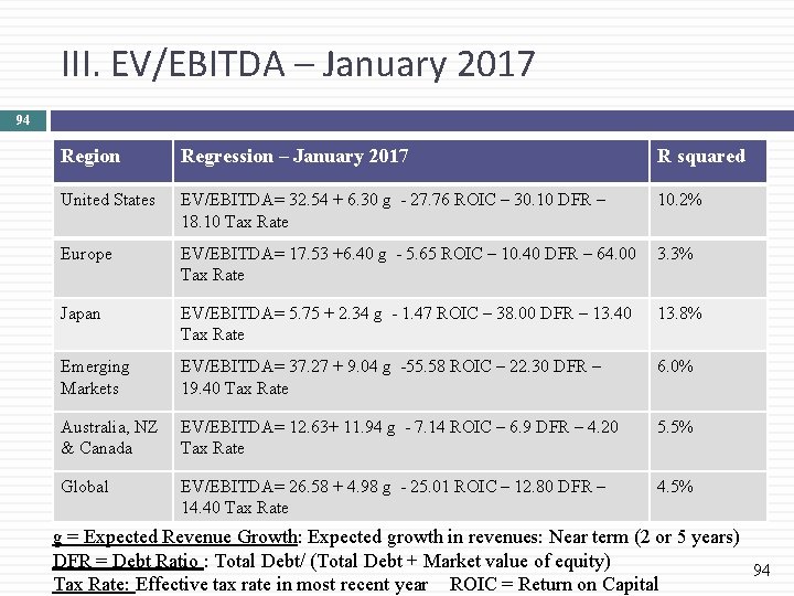
III. EV/EBITDA – January 2017 94 Region Regression – January 2017 R squared United States EV/EBITDA= 32. 54 + 6. 30 g - 27. 76 ROIC – 30. 10 DFR – 18. 10 Tax Rate 10. 2% Europe EV/EBITDA= 17. 53 +6. 40 g - 5. 65 ROIC – 10. 40 DFR – 64. 00 3. 3% Tax Rate Japan EV/EBITDA= 5. 75 + 2. 34 g - 1. 47 ROIC – 38. 00 DFR – 13. 40 Tax Rate 13. 8% Emerging Markets EV/EBITDA= 37. 27 + 9. 04 g -55. 58 ROIC – 22. 30 DFR – 19. 40 Tax Rate 6. 0% Australia, NZ & Canada EV/EBITDA= 12. 63+ 11. 94 g - 7. 14 ROIC – 6. 9 DFR – 4. 20 Tax Rate 5. 5% Global EV/EBITDA= 26. 58 + 4. 98 g - 25. 01 ROIC – 12. 80 DFR – 14. 40 Tax Rate 4. 5% g = Expected Revenue Growth: Expected growth in revenues: Near term (2 or 5 years) DFR = Debt Ratio : Total Debt/ (Total Debt + Market value of equity) 94 Tax Rate: Effective tax rate in most recent year ROIC = Return on Capital

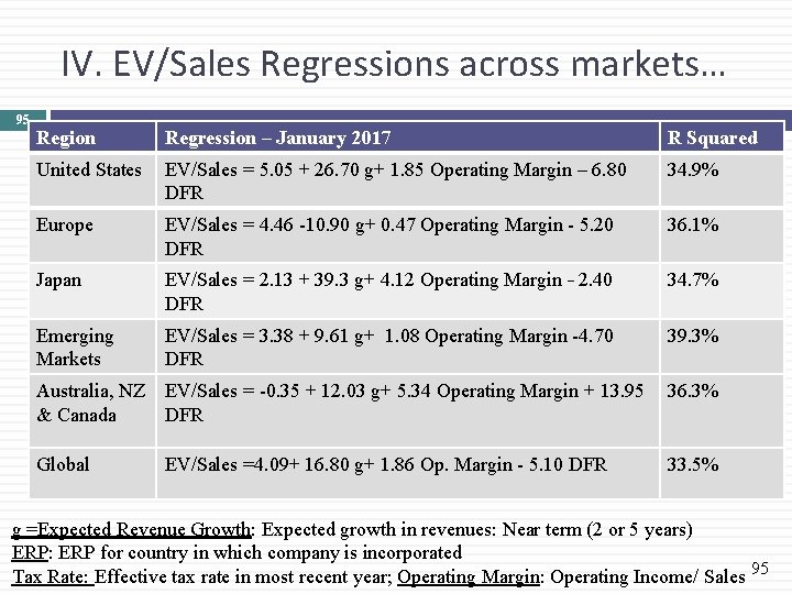
IV. EV/Sales Regressions across markets… 95 Region Regression – January 2017 R Squared United States EV/Sales = 5. 05 + 26. 70 g+ 1. 85 Operating Margin – 6. 80 DFR 34. 9% Europe EV/Sales = 4. 46 -10. 90 g+ 0. 47 Operating Margin - 5. 20 DFR 36. 1% Japan EV/Sales = 2. 13 + 39. 3 g+ 4. 12 Operating Margin – 2. 40 DFR 34. 7% Emerging Markets EV/Sales = 3. 38 + 9. 61 g+ 1. 08 Operating Margin -4. 70 DFR 39. 3% Australia, NZ EV/Sales = -0. 35 + 12. 03 g+ 5. 34 Operating Margin + 13. 95 36. 3% & Canada DFR Global EV/Sales =4. 09+ 16. 80 g+ 1. 86 Op. Margin - 5. 10 DFR 33. 5% g =Expected Revenue Growth: Expected growth in revenues: Near term (2 or 5 years) ERP: ERP for country in which company is incorporated Tax Rate: Effective tax rate in most recent year; Operating Margin: Operating Income/ Sales 95

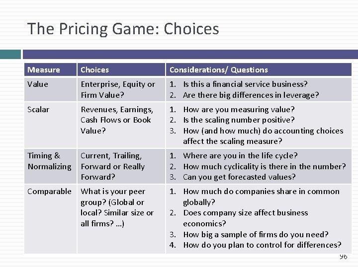
The Pricing Game: Choices Measure Choices Considerations/ Questions Value Enterprise, Equity or Firm Value? 1. Is this a financial service business? 2. Are there big differences in leverage? Scalar Revenues, Earnings, Cash Flows or Book Value? 1. How are you measuring value? 2. Is the scaling number positive? 3. How (and how much) do accounting choices affect the scaling measure? Timing & Normalizing Current, Trailing, Forward or Really Forward? 1. Where are you in the life cycle? 2. How much cyclicality is there in the number? 3. Can you get forecasted values? Comparable What is your peer group? (Global or local? Similar size or all firms? …) Aswath Damodaran 1. How much do companies share in common globally? 2. Does company size affect business economics? 3. How big a sample of firms do you need? 4. How do you plan to control for differences? 96

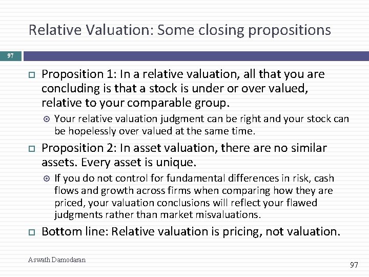
Relative Valuation: Some closing propositions 97 Proposition 1: In a relative valuation, all that you are concluding is that a stock is under or over valued, relative to your comparable group. Proposition 2: In asset valuation, there are no similar assets. Every asset is unique. Your relative valuation judgment can be right and your stock can be hopelessly over valued at the same time. If you do not control for fundamental differences in risk, cash flows and growth across firms when comparing how they are priced, your valuation conclusions will reflect your flawed judgments rather than market misvaluations. Bottom line: Relative valuation is pricing, not valuation. Aswath Damodaran 97

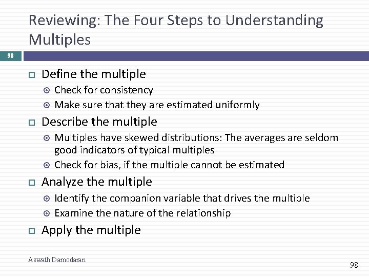
Reviewing: The Four Steps to Understanding Multiples 98 Define the multiple Describe the multiple Multiples have skewed distributions: The averages are seldom good indicators of typical multiples Check for bias, if the multiple cannot be estimated Analyze the multiple Check for consistency Make sure that they are estimated uniformly Identify the companion variable that drives the multiple Examine the nature of the relationship Apply the multiple Aswath Damodaran 98

Aswath Damodaran A DETOUR: ASSET BASED VALUATION Value assets, not cash flows? 99

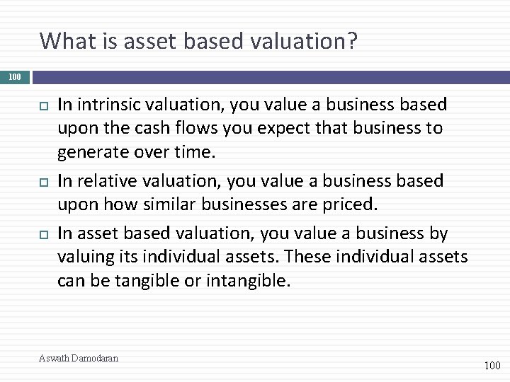
What is asset based valuation? 100 In intrinsic valuation, you value a business based upon the cash flows you expect that business to generate over time. In relative valuation, you value a business based upon how similar businesses are priced. In asset based valuation, you value a business by valuing its individual assets. These individual assets can be tangible or intangible. Aswath Damodaran 100

Why would you do asset based valuation? 101 Liquidation: If you are liquidating a business by selling its assets piece meal, rather than as a composite business, you would like to estimate what you will get from each asset or asset class individually. Accounting mission: As both US and international accounting standards have turned to “fair value” accounting, accountants have been called upon to redo balance sheet to reflect the assets at their fair rather than book value. Sum of the parts: If a business is made up of individual divisions or assets, you may want to value these parts individually for one of two groups: Potential acquirers may want to do this, as a precursor to restructuring the business. Investors may be interested because a business that is selling for less than the sum of its parts may be “cheap”. Aswath Damodaran 101

How do you do asset based valuation? 102 Intrinsic value: Estimate the expected cash flows on each asset or asset class, discount back at a risk adjusted discount rate and arrive at an intrinsic value for each asset. Relative value: Look for similar assets that have sold in the recent past and estimate a value for each asset in the business. Accounting value: You could use the book value of the asset as a proxy for the estimated value of the asset. Aswath Damodaran 102

When is asset-based valuation easiest to do? 103 Separable assets: If a company is a collection of separable assets (a set of real estate holdings, a holding company of different independent businesses), asset-based valuation is easier to do. If the assets are interrelated or difficult to separate, asset-based valuation becomes problematic. Thus, while real estate or a long term licensing/franchising contract may be easily valued, brand name (which cuts across assets) is more difficult to value separately. Stand alone earnings/ cash flows: An asset is much simpler to value if you can trace its earnings/cash flows to it. It is much more difficult to value when the business generates earnings, but the role of individual assets in generating these earnings cannot be isolated. Active market for similar assets: If you plan to do a relative valuation, it is easier if you can find an active market for “similar” assets which you can draw on for transactions prices. Aswath Damodaran 103

I. Liquidation Valuation 104 In liquidation valuation, you are trying to assess how much you would get from selling the assets of the business today, rather than the business as a going concern. Consequently, it makes more sense to price those assets (i. e. , do relative valuation) than it is to value them (do intrinsic valuation). For assets that are separable and traded (example: real estate), pricing is easy to do. For assets that are not, you often see book value used either as a proxy for liquidation value or as a basis for estimating liquidation value. To the extent that the liquidation is urgent, you may attach a discount to the estimated value. Aswath Damodaran 104

II. Accounting Valuation: Glimmers from FAS 157 105 The ubiquitous “market participant”: Through FAS 157, accountants are asked to attach values to assets/liabilities that market participants would have been willing to pay/ receive. Tilt towards relative value: “The definition focuses on the price that would be received to sell the asset or paid to transfer the liability (an exit price), not the price that would be paid to acquire the asset or received to assume the liability (an entry price). ” The hierarchy puts “market prices”, if available for an asset, at the top with intrinsic value being accepted only if market prices are not accessible. Split mission: While accounting fair value is titled towards relative valuation, accountants are also required to back their relative valuations with intrinsic valuations. Often, this leads to reverse engineering, where accountants arrive at values first and develop valuations later. Aswath Damodaran 105

III. Sum of the parts valuation 106 You can value a company in pieces, using either relative or intrinsic valuation. Which one you use will depend on who you are and your motives for doing the sum of the parts valuation. If you are long term, passive investor in the company, your intent may be to find market mistakes that you hope will get corrected over time. If that is the case, you should do an intrinsic valuation of the individual assets. If you are an activist investor that plans to acquire the company or push for change, you should be more focused on relative valuation, since your intent is to get the company to split up and gain the increase in value. Aswath Damodaran 106

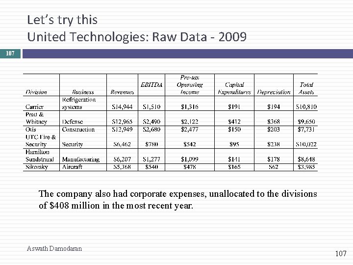
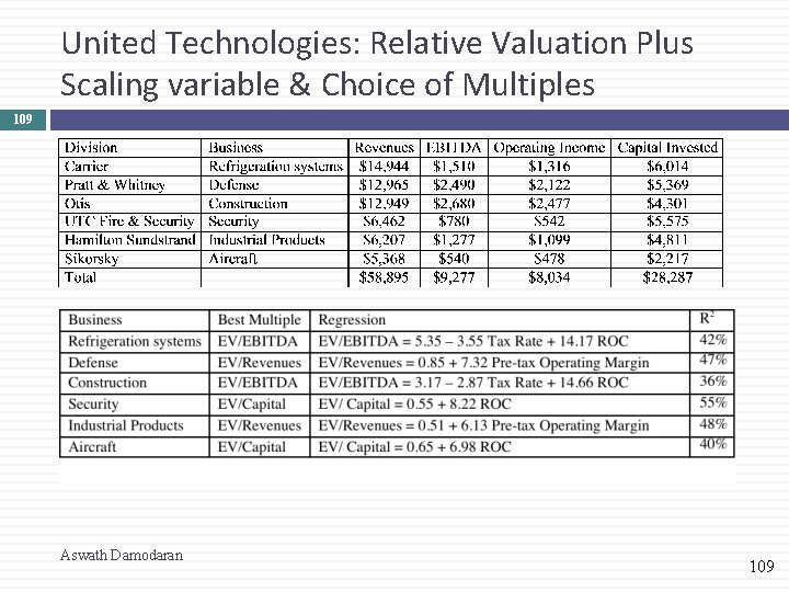
Let’s try this United Technologies: Raw Data - 2009 107 The company also had corporate expenses, unallocated to the divisions of $408 million in the most recent year. Aswath Damodaran 107

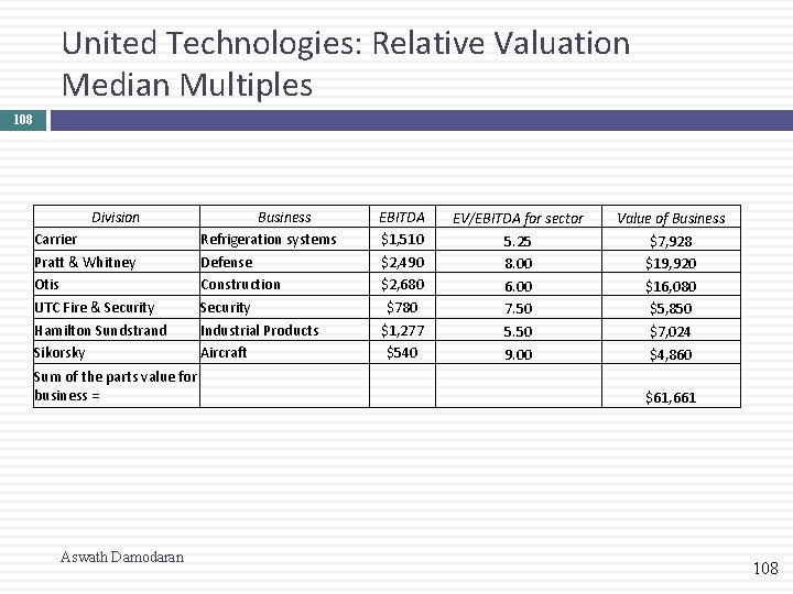
United Technologies: Relative Valuation Median Multiples 108 Division Carrier Pratt & Whitney Otis UTC Fire & Security Hamilton Sundstrand Sikorsky Sum of the parts value for business = Aswath Damodaran Business Refrigeration systems Defense Construction Security Industrial Products Aircraft EBITDA $1, 510 $2, 490 $2, 680 $780 $1, 277 $540 EV/EBITDA for sector 5. 25 8. 00 6. 00 7. 50 5. 50 9. 00 Value of Business $7, 928 $19, 920 $16, 080 $5, 850 $7, 024 $4, 860 $61, 661 108

United Technologies: Relative Valuation Plus Scaling variable & Choice of Multiples 109 Aswath Damodaran 109

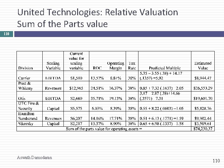
United Technologies: Relative Valuation Sum of the Parts value 110 Aswath Damodaran 110

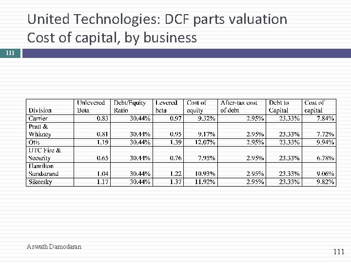
United Technologies: DCF parts valuation Cost of capital, by business 111 Aswath Damodaran 111

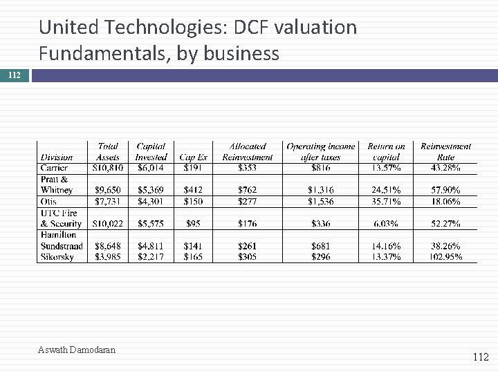
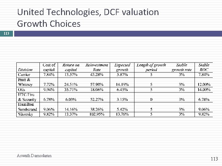
United Technologies: DCF valuation Fundamentals, by business 112 Aswath Damodaran 112

United Technologies, DCF valuation Growth Choices 113 Aswath Damodaran 113

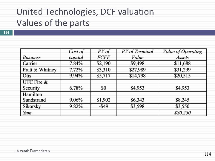
United Technologies, DCF valuation Values of the parts 114 Aswath Damodaran 114

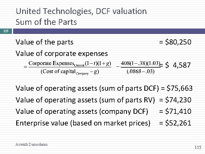
United Technologies, DCF valuation Sum of the Parts 115 Value of the parts Value of corporate expenses = $80, 250 = $ 4, 587 Value of operating assets (sum of parts DCF) = $75, 663 Value of operating assets (sum of parts RV) = $74, 230 Value of operating assets (company DCF) = $71, 410 Enterprise value (based on market prices) = $52, 261 Aswath Damodaran 115

Aswath Damodaran 116 PRIVATE COMPANY VALUATION Aswath Damodaran

Process of Valuing Private Companies 117 The process of valuing private companies is not different from the process of valuing public companies. You estimate cash flows, attach a discount rate based upon the riskiness of the cash flows and compute a present value. As with public companies, you can either value The entire business, by discounting cash flows to the firm at the cost of capital. The equity in the business, by discounting cashflows to equity at the cost of equity. When valuing private companies, you face two standard problems: There is not market value for either debt or equity The financial statements for private firms are likely to go back fewer years, have less detail and have more holes in them. Aswath Damodaran 117

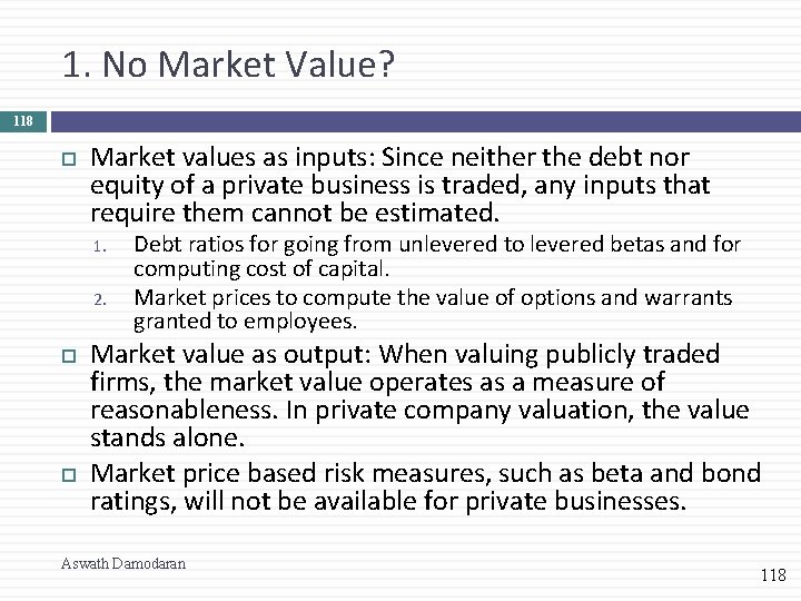
1. No Market Value? 118 Market values as inputs: Since neither the debt nor equity of a private business is traded, any inputs that require them cannot be estimated. 1. 2. Debt ratios for going from unlevered to levered betas and for computing cost of capital. Market prices to compute the value of options and warrants granted to employees. Market value as output: When valuing publicly traded firms, the market value operates as a measure of reasonableness. In private company valuation, the value stands alone. Market price based risk measures, such as beta and bond ratings, will not be available for private businesses. Aswath Damodaran 118

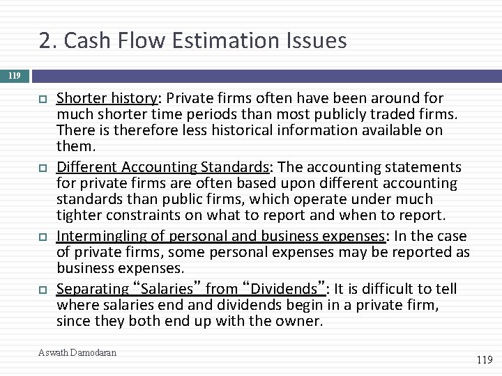
2. Cash Flow Estimation Issues 119 Shorter history: Private firms often have been around for much shorter time periods than most publicly traded firms. There is therefore less historical information available on them. Different Accounting Standards: The accounting statements for private firms are often based upon different accounting standards than public firms, which operate under much tighter constraints on what to report and when to report. Intermingling of personal and business expenses: In the case of private firms, some personal expenses may be reported as business expenses. Separating “Salaries” from “Dividends”: It is difficult to tell where salaries end and dividends begin in a private firm, since they both end up with the owner. Aswath Damodaran 119

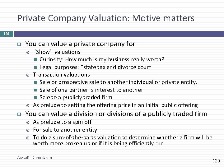
Private Company Valuation: Motive matters 120 You can value a private company for ‘Show’ valuations Curiosity: How much is my business really worth? Legal purposes: Estate tax and divorce court Transaction valuations Sale or prospective sale to another individual or private entity. Sale of one partner’s interest to another Sale to a publicly traded firm As prelude to setting the offering price in an initial public offering You can value a division or divisions of a publicly traded firm As prelude to a spin off For sale to another entity To do a sum-of-the-parts valuation to determine whether a firm will be worth more broken up or if it is being efficiently run. Aswath Damodaran 120

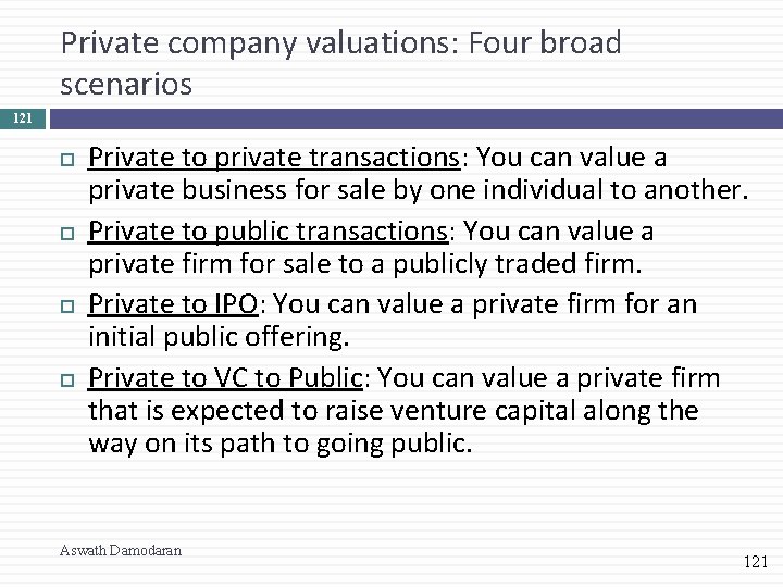
Private company valuations: Four broad scenarios 121 Private to private transactions: You can value a private business for sale by one individual to another. Private to public transactions: You can value a private firm for sale to a publicly traded firm. Private to IPO: You can value a private firm for an initial public offering. Private to VC to Public: You can value a private firm that is expected to raise venture capital along the way on its path to going public. Aswath Damodaran 121

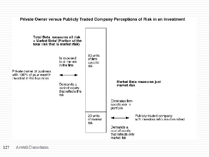
I. Private to Private transaction 122 In private to private transactions, a private business is sold by one individual to another. There are three key issues that we need to confront in such transactions: Neither the buyer nor the seller is diversified. Consequently, risk and return models that focus on just the risk that cannot be diversified away will seriously under estimate the discount rates. The investment is illiquid. Consequently, the buyer of the business will have to factor in an “illiquidity discount” to estimate the value of the business. Key person value: There may be a significant personal component to the value. In other words, the revenues and operating profit of the business reflect not just the potential of the business but the presence of the current owner. Aswath Damodaran 122

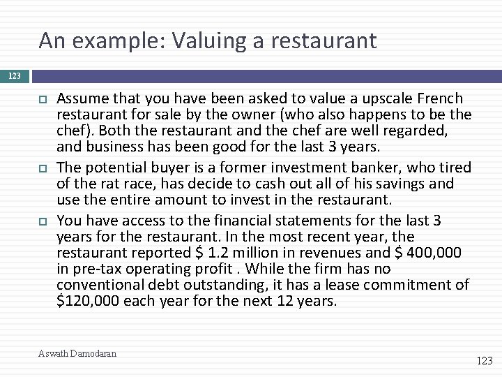
An example: Valuing a restaurant 123 Assume that you have been asked to value a upscale French restaurant for sale by the owner (who also happens to be the chef). Both the restaurant and the chef are well regarded, and business has been good for the last 3 years. The potential buyer is a former investment banker, who tired of the rat race, has decide to cash out all of his savings and use the entire amount to invest in the restaurant. You have access to the financial statements for the last 3 years for the restaurant. In the most recent year, the restaurant reported $ 1. 2 million in revenues and $ 400, 000 in pre-tax operating profit. While the firm has no conventional debt outstanding, it has a lease commitment of $120, 000 each year for the next 12 years. Aswath Damodaran 123

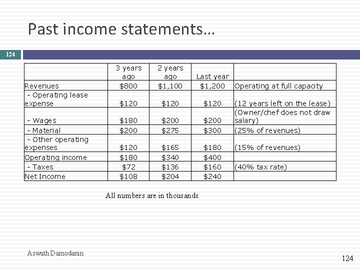
Past income statements… 124 Revenues - Operating lease expense - Wages - Material - Other operating expenses Operating income - Taxes Net Income 3 years ago $800 2 years ago $1, 100 $120 $180 $200 $275 $200 $300 (12 years left on the lease) (Owner/chef does not draw salary) (25% of revenues) $120 $180 $72 $108 $165 $340 $136 $204 $180 $400 $160 $240 (15% of revenues) (40% tax rate) Last year $1, 200 Operating at full capacity All numbers are in thousands Aswath Damodaran 124

Step 1: Estimating discount rates 125 Conventional risk and return models in finance are built on the presumption that the marginal investors in the company are diversified and that they therefore care only about the risk that cannot be diversified. That risk is measured with a beta or betas, usually estimated by looking at past prices or returns. In this valuation, both assumptions are likely to be violated: As a private business, this restaurant has no market prices or returns to use in estimation. The buyer is not diversified. In fact, he will have his entire wealth tied up in the restaurant after the purchase. Aswath Damodaran 125

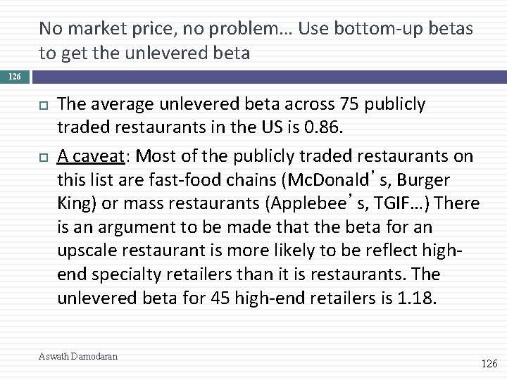
No market price, no problem… Use bottom-up betas to get the unlevered beta 126 The average unlevered beta across 75 publicly traded restaurants in the US is 0. 86. A caveat: Most of the publicly traded restaurants on this list are fast-food chains (Mc. Donald’s, Burger King) or mass restaurants (Applebee’s, TGIF…) There is an argument to be made that the beta for an upscale restaurant is more likely to be reflect highend specialty retailers than it is restaurants. The unlevered beta for 45 high-end retailers is 1. 18. Aswath Damodaran 126

127 Aswath Damodaran

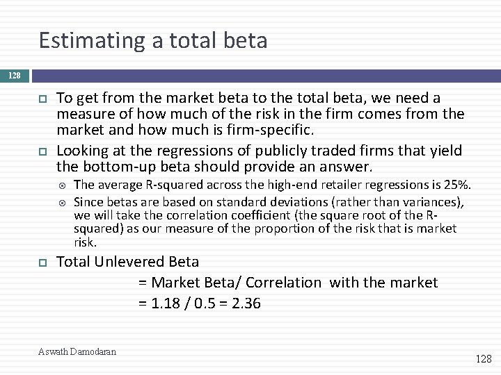
Estimating a total beta 128 To get from the market beta to the total beta, we need a measure of how much of the risk in the firm comes from the market and how much is firm-specific. Looking at the regressions of publicly traded firms that yield the bottom-up beta should provide an answer. The average R-squared across the high-end retailer regressions is 25%. Since betas are based on standard deviations (rather than variances), we will take the correlation coefficient (the square root of the Rsquared) as our measure of the proportion of the risk that is market risk. Total Unlevered Beta = Market Beta/ Correlation with the market = 1. 18 / 0. 5 = 2. 36 Aswath Damodaran 128

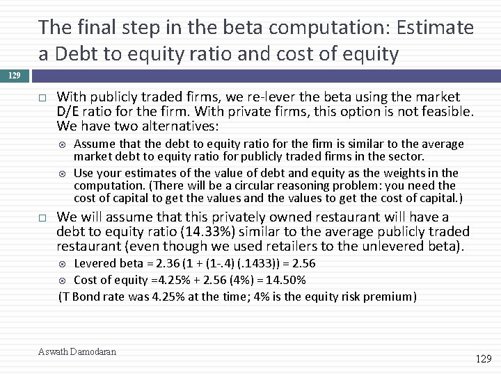
The final step in the beta computation: Estimate a Debt to equity ratio and cost of equity 129 With publicly traded firms, we re-lever the beta using the market D/E ratio for the firm. With private firms, this option is not feasible. We have two alternatives: Assume that the debt to equity ratio for the firm is similar to the average market debt to equity ratio for publicly traded firms in the sector. Use your estimates of the value of debt and equity as the weights in the computation. (There will be a circular reasoning problem: you need the cost of capital to get the values and the values to get the cost of capital. ) We will assume that this privately owned restaurant will have a debt to equity ratio (14. 33%) similar to the average publicly traded restaurant (even though we used retailers to the unlevered beta). Levered beta = 2. 36 (1 + (1 -. 4) (. 1433)) = 2. 56 Cost of equity =4. 25% + 2. 56 (4%) = 14. 50% (T Bond rate was 4. 25% at the time; 4% is the equity risk premium) Aswath Damodaran 129

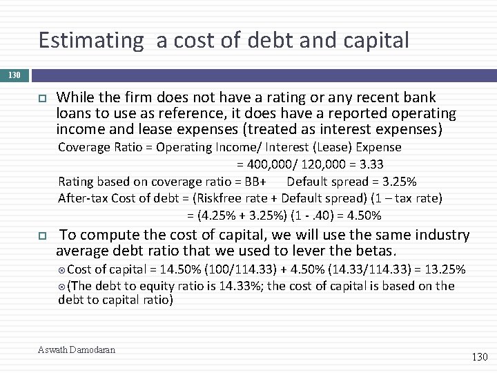
Estimating a cost of debt and capital 130 While the firm does not have a rating or any recent bank loans to use as reference, it does have a reported operating income and lease expenses (treated as interest expenses) Coverage Ratio = Operating Income/ Interest (Lease) Expense = 400, 000/ 120, 000 = 3. 33 Rating based on coverage ratio = BB+ Default spread = 3. 25% After-tax Cost of debt = (Riskfree rate + Default spread) (1 – tax rate) = (4. 25% + 3. 25%) (1 -. 40) = 4. 50% To compute the cost of capital, we will use the same industry average debt ratio that we used to lever the betas. Cost of capital = 14. 50% (100/114. 33) + 4. 50% (14. 33/114. 33) = 13. 25% (The debt to equity ratio is 14. 33%; the cost of capital is based on the debt to capital ratio) Aswath Damodaran 130

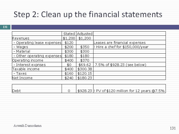
Step 2: Clean up the financial statements 131 Revenues - Operating lease expenses - Wages - Material - Other operating expenses Operating income - Interest expnses Taxable income - Taxes Net Income Debt Aswath Damodaran Stated $1, 200 $120 $200 $300 $180 $400 $160 $240 0 Adjusted $1, 200 $350 $300 $180 $370 $69. 62 $300. 38 $120. 15 $180. 23 Leases are financial expenses ! Hire a chef for $150, 000/year 7. 5% of $928. 23 (see below) $928. 23 ! PV of $120 million for 12 years @7. 5% 131

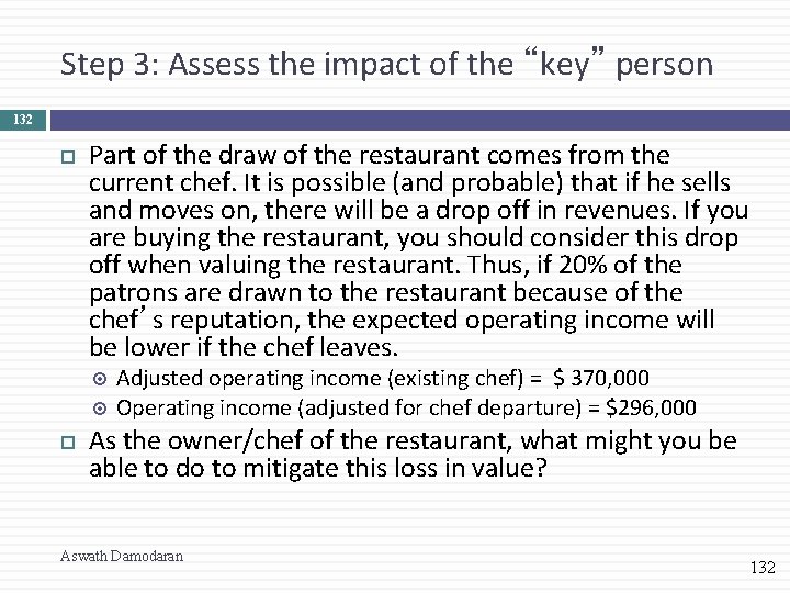
Step 3: Assess the impact of the “key” person 132 Part of the draw of the restaurant comes from the current chef. It is possible (and probable) that if he sells and moves on, there will be a drop off in revenues. If you are buying the restaurant, you should consider this drop off when valuing the restaurant. Thus, if 20% of the patrons are drawn to the restaurant because of the chef’s reputation, the expected operating income will be lower if the chef leaves. Adjusted operating income (existing chef) = $ 370, 000 Operating income (adjusted for chef departure) = $296, 000 As the owner/chef of the restaurant, what might you be able to do to mitigate this loss in value? Aswath Damodaran 132

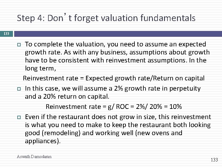
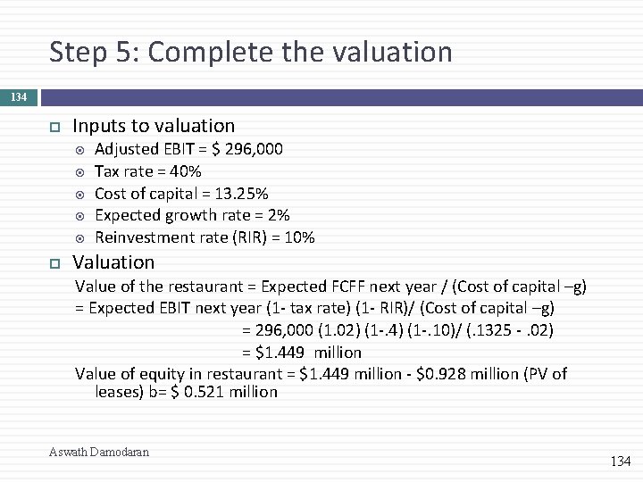
Step 4: Don’t forget valuation fundamentals 133 To complete the valuation, you need to assume an expected growth rate. As with any business, assumptions about growth have to be consistent with reinvestment assumptions. In the long term, Reinvestment rate = Expected growth rate/Return on capital In this case, we will assume a 2% growth rate in perpetuity and a 20% return on capital. Reinvestment rate = g/ ROC = 2%/ 20% = 10% Even if the restaurant does not grow in size, this reinvestment is what you need to make to keep the restaurant both looking good (remodeling) and working well (new ovens and appliances). Aswath Damodaran 133

Step 5: Complete the valuation 134 Inputs to valuation Adjusted EBIT = $ 296, 000 Tax rate = 40% Cost of capital = 13. 25% Expected growth rate = 2% Reinvestment rate (RIR) = 10% Valuation Value of the restaurant = Expected FCFF next year / (Cost of capital –g) = Expected EBIT next year (1 - tax rate) (1 - RIR)/ (Cost of capital –g) = 296, 000 (1. 02) (1 -. 4) (1 -. 10)/ (. 1325 -. 02) = $1. 449 million Value of equity in restaurant = $1. 449 million - $0. 928 million (PV of leases) b= $ 0. 521 million Aswath Damodaran 134

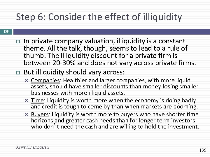
Step 6: Consider the effect of illiquidity 135 In private company valuation, illiquidity is a constant theme. All the talk, though, seems to lead to a rule of thumb. The illiquidity discount for a private firm is between 20 -30% and does not vary across private firms. But illiquidity should vary across: Companies: Healthier and larger companies, with more liquid assets, should have smaller discounts than money-losing smaller businesses with more illiquid assets. Time: Liquidity is worth more when the economy is doing badly and credit is tough to come by than when markets are booming. Buyers: Liquidity is worth more to buyers who have shorter time horizons and greater cash needs than for longer term investors who don’t need the cash and are willing to hold the investment. Aswath Damodaran 135

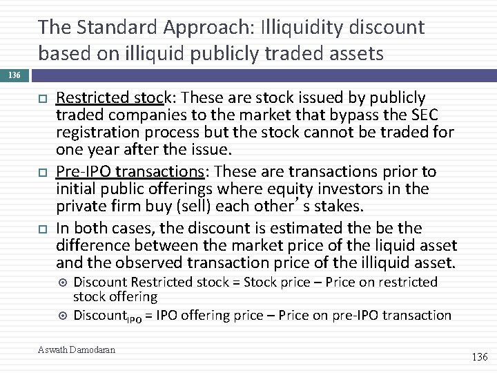
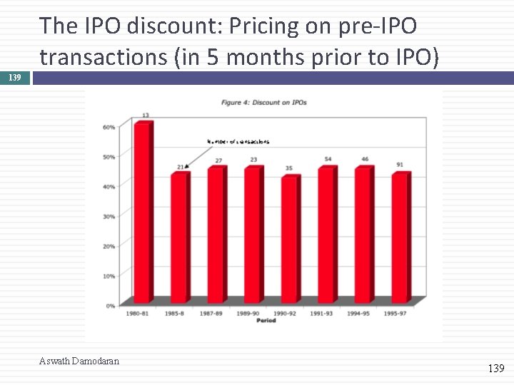
The Standard Approach: Illiquidity discount based on illiquid publicly traded assets 136 Restricted stock: These are stock issued by publicly traded companies to the market that bypass the SEC registration process but the stock cannot be traded for one year after the issue. Pre-IPO transactions: These are transactions prior to initial public offerings where equity investors in the private firm buy (sell) each other’s stakes. In both cases, the discount is estimated the be the difference between the market price of the liquid asset and the observed transaction price of the illiquid asset. Discount Restricted stock = Stock price – Price on restricted stock offering Discount. IPO = IPO offering price – Price on pre-IPO transaction Aswath Damodaran 136

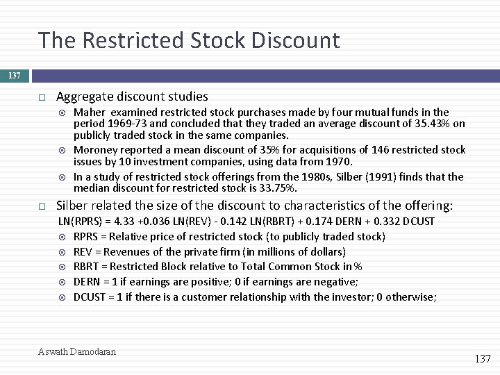
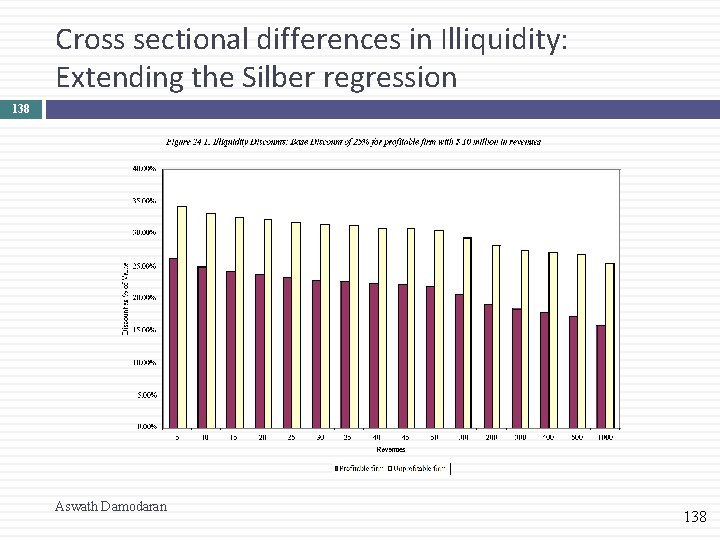
The Restricted Stock Discount 137 Aggregate discount studies Maher examined restricted stock purchases made by four mutual funds in the period 1969 -73 and concluded that they traded an average discount of 35. 43% on publicly traded stock in the same companies. Moroney reported a mean discount of 35% for acquisitions of 146 restricted stock issues by 10 investment companies, using data from 1970. In a study of restricted stock offerings from the 1980 s, Silber (1991) finds that the median discount for restricted stock is 33. 75%. Silber related the size of the discount to characteristics of the offering: LN(RPRS) = 4. 33 +0. 036 LN(REV) - 0. 142 LN(RBRT) + 0. 174 DERN + 0. 332 DCUST RPRS = Relative price of restricted stock (to publicly traded stock) REV = Revenues of the private firm (in millions of dollars) RBRT = Restricted Block relative to Total Common Stock in % DERN = 1 if earnings are positive; 0 if earnings are negative; DCUST = 1 if there is a customer relationship with the investor; 0 otherwise; Aswath Damodaran 137

Cross sectional differences in Illiquidity: Extending the Silber regression 138 Aswath Damodaran 138

The IPO discount: Pricing on pre-IPO transactions (in 5 months prior to IPO) 139 Aswath Damodaran 139

The “sampling” problem 140 With both restricted stock and the IPO studies, there is a significant sampling bias problem. The companies that make restricted stock offerings are likely to be small, troubled firms that have run out of conventional financing options. The types of IPOs where equity investors sell their stake in the five months prior to the IPO at a huge discount are likely to be IPOs that have significant pricing uncertainty associated with them. With restricted stock, the magnitude of the sampling bias was estimated by comparing the discount on all private placements to the discount on restricted stock offerings. One study concluded that the “illiquidity” alone accounted for a discount of less than 10% (leaving the balance of 20 -25% to be explained by sampling problems). Aswath Damodaran 140

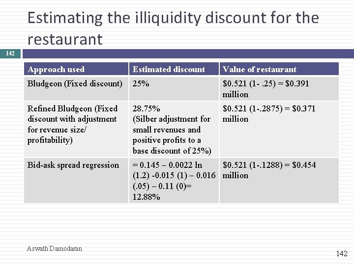
An alternative approach: Use the whole sample 141 All traded assets are illiquid. The bid ask spread, measuring the difference between the price at which you can buy and sell the asset at the same point in time is the illiquidity measure. We can regress the bid-ask spread (as a percent of the price) against variables that can be measured for a private firm (such as revenues, cash flow generating capacity, type of assets, variance in operating income) and are also available for publicly traded firms. Using data from the end of 2000, for instance, we regressed the bid -ask spread against annual revenues, a dummy variable for positive earnings (DERN: 0 if negative and 1 if positive), cash as a percent of firm value and trading volume. Spread = 0. 145 – 0. 0022 ln (Annual Revenues) -0. 015 (DERN) – 0. 016 (Cash/Firm Value) – 0. 11 ($ Monthly trading volume/ Firm Value) You could plug in the values for a private firm into this regression (with zero trading volume) and estimate the spread for the firm. Aswath Damodaran 141

Estimating the illiquidity discount for the restaurant 142 Approach used Estimated discount Value of restaurant Bludgeon (Fixed discount) 25% $0. 521 (1 -. 25) = $0. 391 million Refined Bludgeon (Fixed discount with adjustment for revenue size/ profitability) 28. 75% (Silber adjustment for small revenues and positive profits to a base discount of 25%) $0. 521 (1 -. 2875) = $0. 371 million Bid-ask spread regression = 0. 145 – 0. 0022 ln $0. 521 (1 -. 1288) = $0. 454 (1. 2) -0. 015 (1) – 0. 016 million (. 05) – 0. 11 (0)= 12. 88% Aswath Damodaran 142

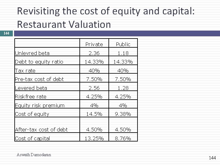
II. Private company sold to publicly traded company 143 The key difference between this scenario and the previous scenario is that the seller of the business is not diversified but the buyer is (or at least the investors in the buyer are). Consequently, they can look at the same firm and see very different amounts of risk in the business with the seller seeing more risk than the buyer. The cash flows may also be affected by the fact that the tax rates for publicly traded companies can diverge from those of private owners. Finally, there should be no illiquidity discount to a public buyer, since investors in the buyer can sell their holdings in a market. Aswath Damodaran 143

Revisiting the cost of equity and capital: Restaurant Valuation 144 Private Public 2. 36 1. 18 14. 33% 40% 7. 50% Levered beta 2. 56 1. 28 Riskfree rate 4. 25% 4% 4% Cost of equity 14. 5% 9. 38% After-tax cost of debt 4. 50% 13. 25% 8. 76% Unlevred beta Debt to equity ratio Tax rate Pre-tax cost of debt Equity risk premium Cost of capital Aswath Damodaran 144

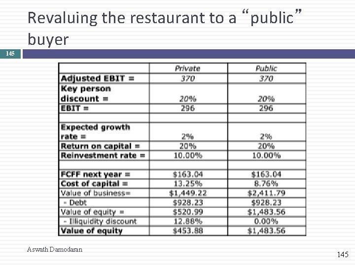
Revaluing the restaurant to a “public” buyer 145 Aswath Damodaran 145

So, what price should you ask for? 146 a. b. c. Assume that you represent the chef/owner of the restaurant and that you were asking for a “reasonable” price for the restaurant. What would you ask for? $ 454, 000 $ 1. 484 million Some number in the middle If it is “some number in the middle”, what will determine what you will ultimately get for your business? How would you alter the analysis, if your best potential bidder is a private equity or VC fund rather than a publicly traded firm? Aswath Damodaran 146

III. Private company for initial public offering 147 In an initial public offering, the private business is opened up to investors who clearly are diversified (or at least have the option to be diversified). There are control implications as well. When a private firm goes public, it opens itself up to monitoring by investors, analysts and market. The reporting and information disclosure requirements shift to reflect a publicly traded firm. Aswath Damodaran 147

148 Aswath Damodaran

The twists in an initial public offering 149 Valuation issues: Use of the proceeds from the offering: The proceeds from the offering can be held as cash by the firm to cover future investment needs, paid to existing equity investors who want to cash out or used to pay down debt. Warrants/ Special deals with prior equity investors: If venture capitalists and other equity investors from earlier iterations of fund raising have rights to buy or sell their equity at pre-specified prices, it can affect the value per share offered to the public. Pricing issues: Institutional set-up: Most IPOs are backed by investment banking guarantees on the price, which can affect how they are priced. Follow-up offerings: The proportion of equity being offered at initial offering and subsequent offering plans can affect pricing. Aswath Damodaran 149

A. Use of the Proceeds 150 The proceeds from an initial public offering can be Taken out of the firm by the existing owners Used to pay down debt and other obligations Held as cash by the company to cover future reinvestment needs How you deal with the issuance will depend upon how the proceeds are used. If taken out of the firm -> Ignore in valuation If used to pay down debt -> Change the debt ratio, which may change the cost of capital and the value of the firm If held as cash to cover future reinvestment needs -> Add the cash proceeds from the IPO to the DCF valuation of the company. Aswath Damodaran 150

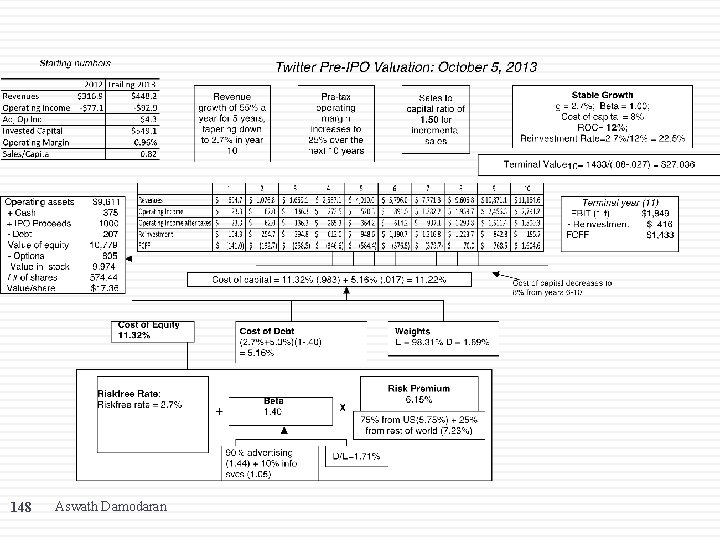
The IPO Proceeds: Twitter 151 How much? News stories suggest that the company is planning on raising about $1 billion from the offering. Use: In the Twitter prospectus filing, the company specifies that it plans to keep the proceeds in the company to meet future investment needs. In the valuation, I have added a billion to the estimated value of the operating assets because that cash infusion will augment the cash balance. How would the valuation have been different if the owners announced that they planned to withdraw half of the offering proceeds? Aswath Damodaran 151

B. Claims from prior equity investors 152 When a private firm goes public, there already equity investors in the firm, including the founder(s), venture capitalists and other equity investors. In some cases, these equity investors can have warrants, options or other special claims on the equity of the firm. If existing equity investors have special claims on the equity, the value of equity per share has to be affected by these claims. Specifically, these options need to be valued at the time of the offering and the value of equity reduced by the option value before determining the value per share. Aswath Damodaran 152

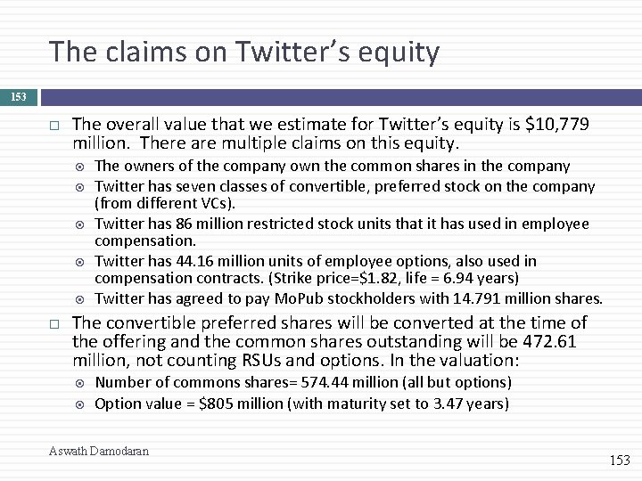
The claims on Twitter’s equity 153 The overall value that we estimate for Twitter’s equity is $10, 779 million. There are multiple claims on this equity. The owners of the company own the common shares in the company Twitter has seven classes of convertible, preferred stock on the company (from different VCs). Twitter has 86 million restricted stock units that it has used in employee compensation. Twitter has 44. 16 million units of employee options, also used in compensation contracts. (Strike price=$1. 82, life = 6. 94 years) Twitter has agreed to pay Mo. Pub stockholders with 14. 791 million shares. The convertible preferred shares will be converted at the time of the offering and the common shares outstanding will be 472. 61 million, not counting RSUs and options. In the valuation: Number of commons shares= 574. 44 million (all but options) Option value = $805 million (with maturity set to 3. 47 years) Aswath Damodaran 153

C. The Investment Banking guarantee… 154 Almost all IPOs are managed by investment banks and are backed by a pricing guarantee, where the investment banker guarantees the offering price to the issuer. If the price at which the issuance is made is lower than the guaranteed price, the investment banker will buy the shares at the guaranteed price and potentially bear the loss. Aswath Damodaran 154

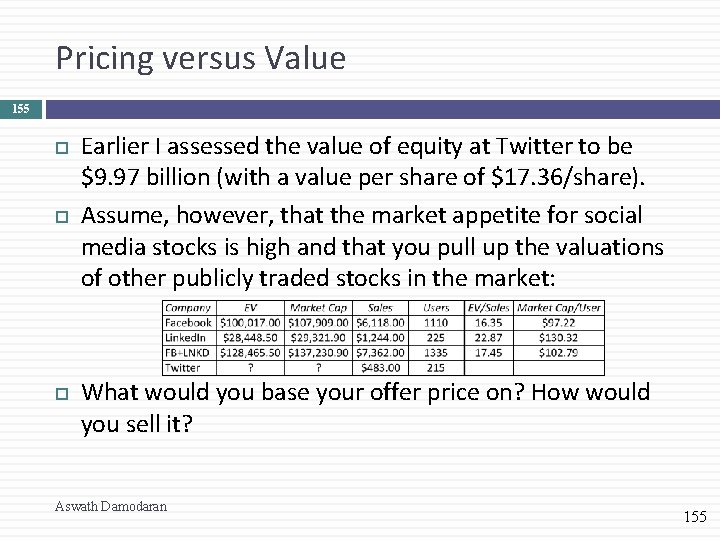
Pricing versus Value 155 Earlier I assessed the value of equity at Twitter to be $9. 97 billion (with a value per share of $17. 36/share). Assume, however, that the market appetite for social media stocks is high and that you pull up the valuations of other publicly traded stocks in the market: What would you base your offer price on? How would you sell it? Aswath Damodaran 155

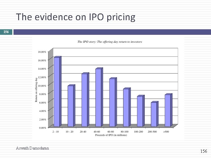
The evidence on IPO pricing 156 Aswath Damodaran 156

An investment opportunity? 157 Assume that investment banks try to under price initial public offerings by approximately 10 -15%. As an investor, what strategy would you adopt to take advantage of this behavior? Why might it not work? Aswath Damodaran 157

D. The offering quantity 158 Assume now that you are the owner of Twitter and were offering 100% of the shares in company in the offering to the public? If investors are willing to pay $20 billion for the common stock, how much do you lose because of the under pricing (15%)? Assume that you were offering only 10% of the shares in the initial offering and plan to sell a large portion of your remaining stake over the following two years? Would your views of the under pricing and its effect on your wealth change as a consequence? Aswath Damodaran 158

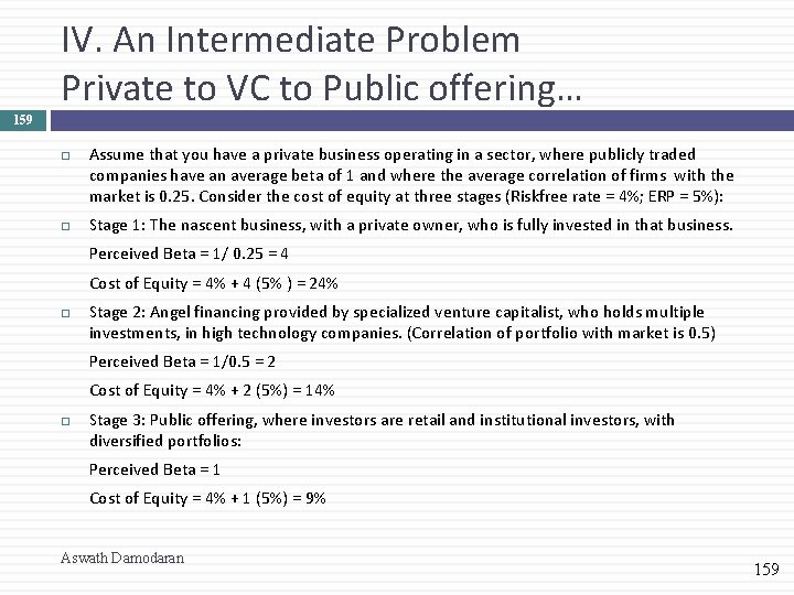
IV. An Intermediate Problem Private to VC to Public offering… 159 Assume that you have a private business operating in a sector, where publicly traded companies have an average beta of 1 and where the average correlation of firms with the market is 0. 25. Consider the cost of equity at three stages (Riskfree rate = 4%; ERP = 5%): Stage 1: The nascent business, with a private owner, who is fully invested in that business. Perceived Beta = 1/ 0. 25 = 4 Cost of Equity = 4% + 4 (5% ) = 24% Stage 2: Angel financing provided by specialized venture capitalist, who holds multiple investments, in high technology companies. (Correlation of portfolio with market is 0. 5) Perceived Beta = 1/0. 5 = 2 Cost of Equity = 4% + 2 (5%) = 14% Stage 3: Public offering, where investors are retail and institutional investors, with diversified portfolios: Perceived Beta = 1 Cost of Equity = 4% + 1 (5%) = 9% Aswath Damodaran 159

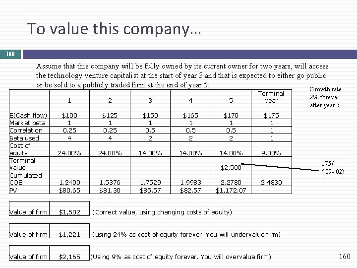
To value this company… 160 Assume that this company will be fully owned by its current owner for two years, will access the technology venture capitalist at the start of year 3 and that is expected to either go public or be sold to a publicly traded firm at the end of year 5. 1 2 3 4 5 Terminal year E(Cash flow) Market beta Correlation Beta used Cost of equity Terminal value Cumulated COE PV $100 1 0. 25 4 $125 1 0. 25 4 $150 1 0. 5 2 $165 1 0. 5 2 $170 1 0. 5 2 $175 1 1 1 24. 00% 14. 00% 9. 00% $2, 500 1. 2400 $80. 65 1. 5376 $81. 30 1. 7529 $85. 57 1. 9983 $82. 57 2. 2780 $1, 172. 07 2. 4830 Value of firm $1, 502 (Correct value, using changing costs of equity) Value of firm $1, 221 (using 24% as cost of equity forever. You will undervalue firm) Value of firm $2, 165 (Using 9% as cost of equity forever. You will overvalue firm) Growth rate 2% forever after year 5 175/ (. 09 -. 02) 160

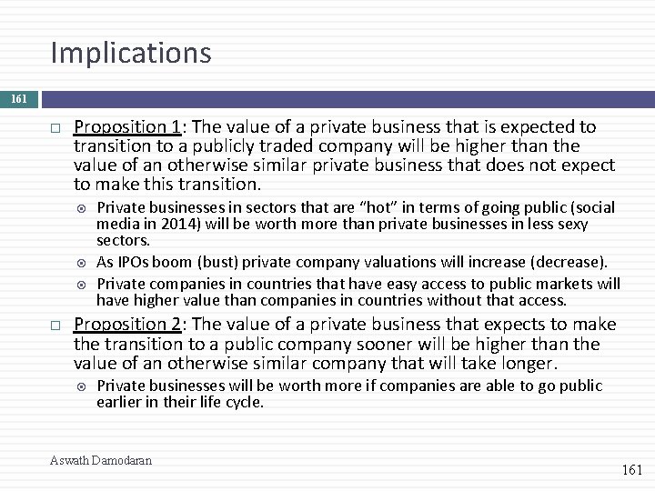
Implications 161 Proposition 1: The value of a private business that is expected to transition to a publicly traded company will be higher than the value of an otherwise similar private business that does not expect to make this transition. Private businesses in sectors that are “hot” in terms of going public (social media in 2014) will be worth more than private businesses in less sexy sectors. As IPOs boom (bust) private company valuations will increase (decrease). Private companies in countries that have easy access to public markets will have higher value than companies in countries without that access. Proposition 2: The value of a private business that expects to make the transition to a public company sooner will be higher than the value of an otherwise similar company that will take longer. Private businesses will be worth more if companies are able to go public earlier in their life cycle. Aswath Damodaran 161

Private company valuation: Closing thoughts 162 The value of a private business will depend on the potential buyer. If you are the seller of a private business, you will maximize value, if you can sell to A long term investor Who is well diversified (or whose investors are) And does not think too highly of you (as a person) If you are valuing a private business for legal purposes (tax or divorce court), the assumptions you use and the value you arrive at will depend on which side of the legal divide you are on. As a final proposition, always keep in mind that the owner of a private business has the option of investing his wealth in publicly traded stocks. There has to be a relationship between what you can earn on those investments and what you demand as a return on your business. Aswath Damodaran 162