Astronomical site evaluation at Dome Fuji on the

Astronomical site evaluation at Dome Fuji on the Antarctic plateau Hirofumi OKITA June 17, 2013 Based on Okita et al. , A&A, 554, L 5 (2013) and some unpublished results /53

Contents 1. Introduction 2. Instrumentations 3. Data processing and error analysis 4. Results 5. Discussion and conclusion 6. Future work 2/53

Contents 1. Introduction 2. Instrumentations 3. Data processing and error analysis 4. Results 5. Discussion and conclusion 6. Future work 3/53

1. 1 Aim of this study The aim of this study is to investigate the astronomical seeing in the free atmosphere above and to determine the height of the surface boundary layer at Dome Fuji on the Antarctic plateau. 4/53

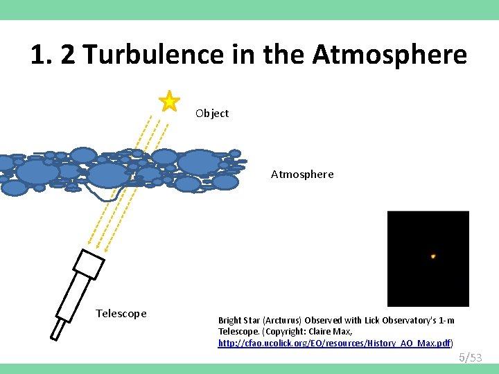
1. 2 Turbulence in the Atmosphere Object Atmosphere Telescope Bright Star (Arcturus) Observed with Lick Observatory's 1 -m Telescope. (Copyright: Claire Max, http: //cfao. ucolick. org/EO/resources/History_AO_Max. pdf) 5/53

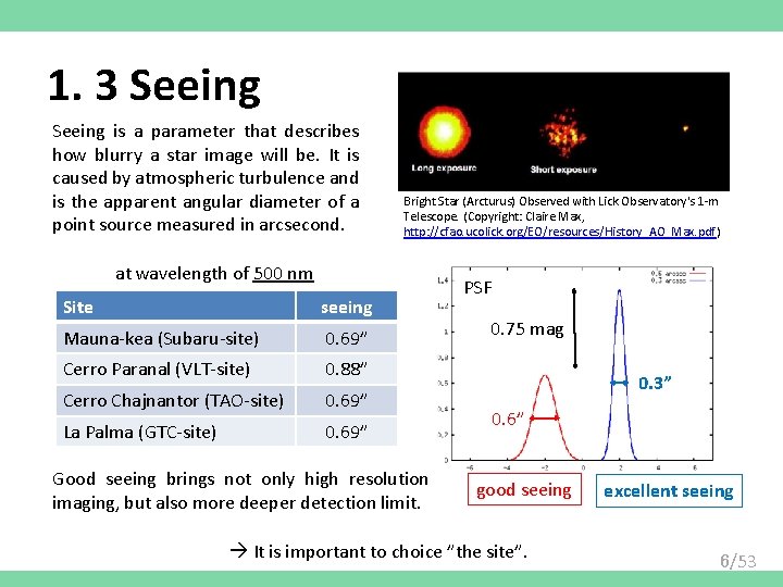
1. 3 Seeing is a parameter that describes how blurry a star image will be. It is caused by atmospheric turbulence and is the apparent angular diameter of a point source measured in arcsecond. Bright Star (Arcturus) Observed with Lick Observatory's 1 -m Telescope. (Copyright: Claire Max, http: //cfao. ucolick. org/EO/resources/History_AO_Max. pdf) at wavelength of 500 nm Site seeing Mauna-kea (Subaru-site) 0. 69” Cerro Paranal (VLT-site) 0. 88” Cerro Chajnantor (TAO-site) 0. 69” La Palma (GTC-site) 0. 69” Good seeing brings not only high resolution imaging, but also more deeper detection limit. PSF 0. 75 mag 0. 3” 0. 6” good seeing It is important to choice ”the site”. excellent seeing 6/53

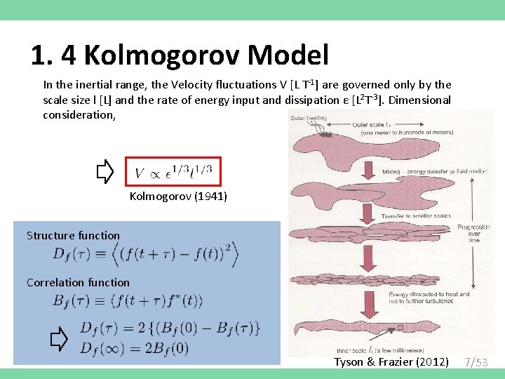
1. 4 Kolmogorov Model In the inertial range, the Velocity fluctuations V [L T-1] are governed only by the scale size l [L] and the rate of energy input and dissipation ε [L 2 T-3]. Dimensional consideration, Kolmogorov (1941) Structure function Correlation function Tyson & Frazier (2012) 7/53

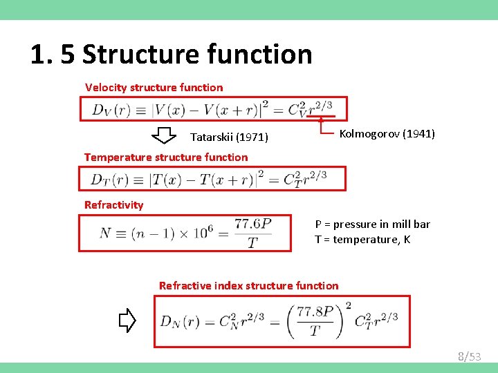
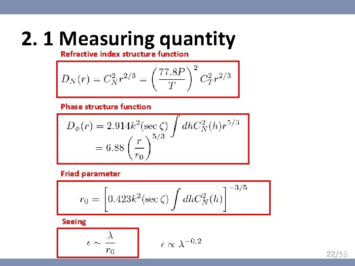
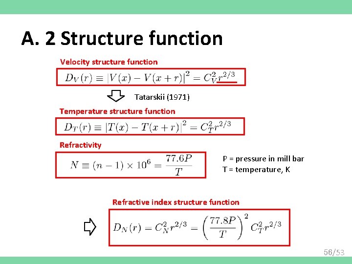
1. 5 Structure function Velocity structure function Tatarskii (1971) Kolmogorov (1941) Temperature structure function Refractivity P = pressure in mill bar T = temperature, K Refractive index structure function 8/53

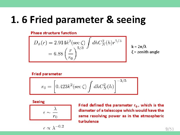
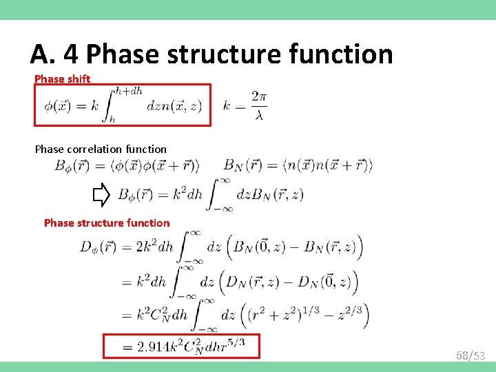
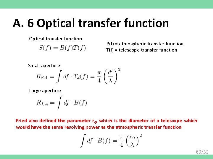
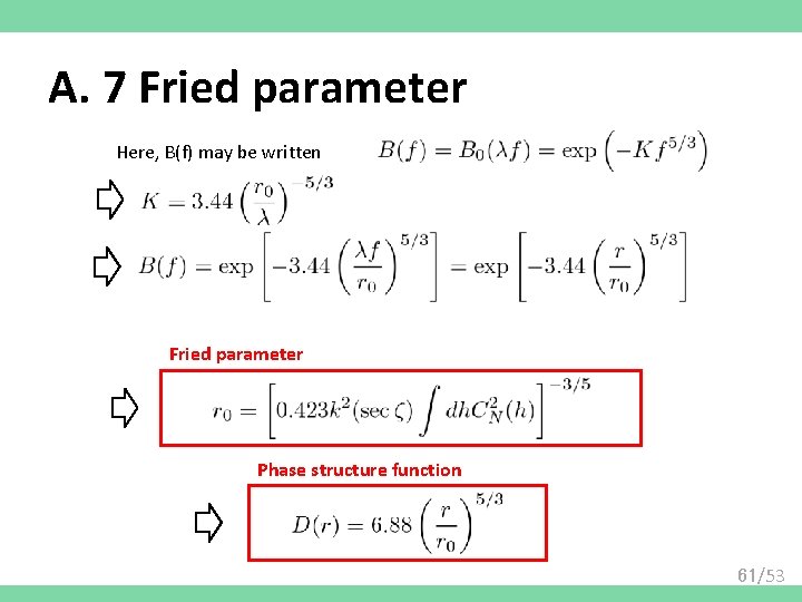
1. 6 Fried parameter & seeing Phase structure function k = 2π/λ ζ = zenith angle Fried parameter Seeing Fried defined the parameter r 0 , which is the diameter of a telescope which would have the same resolving power as in the atmospheric turbulence 9/53

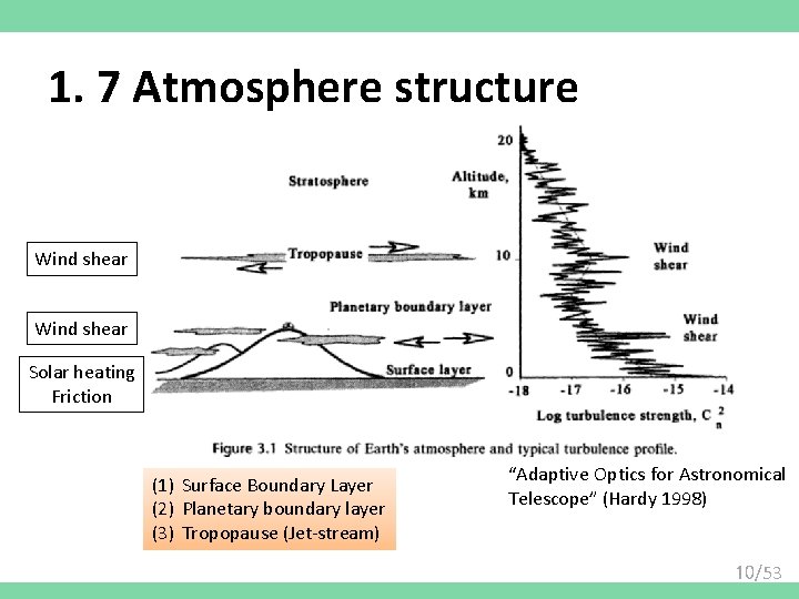
1. 7 Atmosphere structure Wind shear Solar heating Friction (1) Surface Boundary Layer (2) Planetary boundary layer (3) Tropopause (Jet-stream) “Adaptive Optics for Astronomical Telescope” (Hardy 1998) 10/53

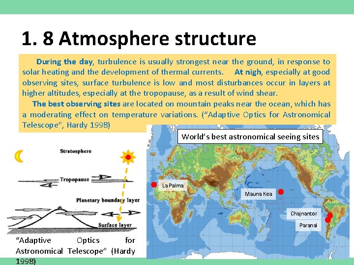
1. 8 Atmosphere structure During the day, turbulence is usually strongest near the ground, in response to solar heating and the development of thermal currents. At nigh, especially at good observing sites, surface turbulence is low and most disturbances occur in layers at higher altitudes, especially at the tropopause, as a result of wind shear. The best observing sites are located on mountain peaks near the ocean, which has a moderating effect on temperature variations. (“Adaptive Optics for Astronomical Telescope”, Hardy 1998) World’s best astronomical seeing sites La Palma Mauna Kea Chajnantor Paranal “Adaptive Optics for Astronomical Telescope” (Hardy 1998) 11/53

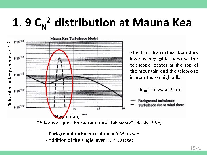
1. 9 CN distribution at Mauna Kea Refractive index parameter CN 2 2 Effect of the surface boundary layer is negligible because the telescope locates at the top of the mountain and the telescope is mounted on high pillar. h. SBL ~ a few x 10 m Height (km) “Adaptive Optics for Astronomical Telescope” (Hardy 1998) - Background turbulence alone = 0. 36 arcsec - Addition of the single layer = 0. 53 arcsec 12/53

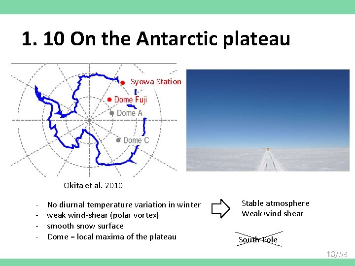
1. 10 On the Antarctic plateau Syowa Station Okita et al. 2010 - No diurnal temperature variation in winter weak wind-shear (polar vortex) smooth snow surface Dome = local maxima of the plateau Stable atmosphere Weak wind shear South Pole 13/53

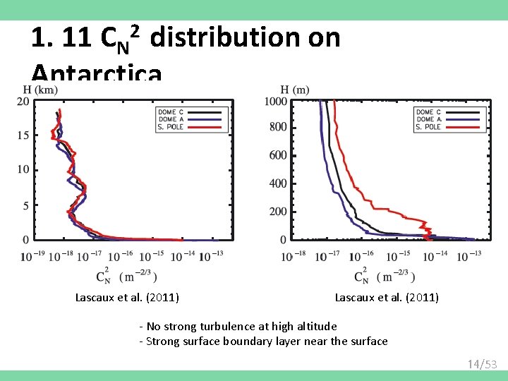
1. 11 CN 2 distribution on Antarctica Lascaux et al. (2011) - No strong turbulence at high altitude - Strong surface boundary layer near the surface 14/53

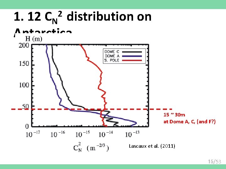
1. 12 CN 2 distribution on Antarctica 15 ~ 30 m at Dome A, C, (and F? ) Lascaux et al. (2011) 15/53

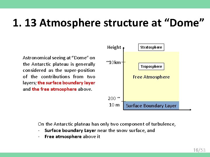
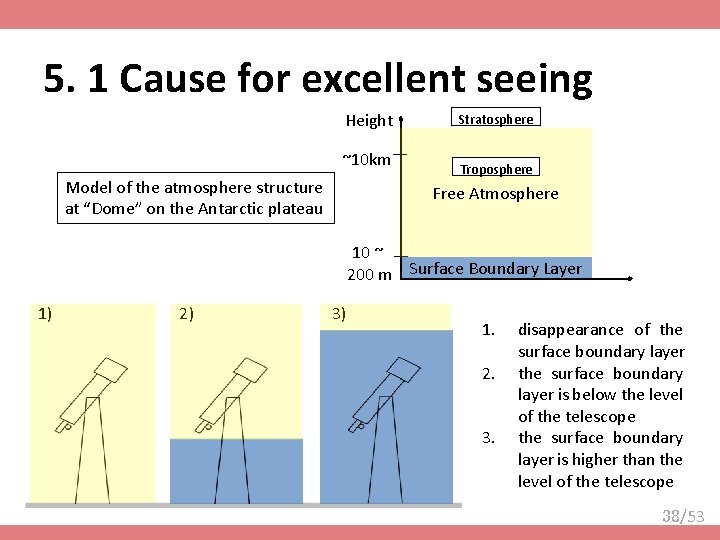
1. 13 Atmosphere structure at “Dome” Height Astronomical seeing at “Dome” on the Antarctic plateau is generally considered as the super-position of the contributions from two layers; the surface boundary layer and the free atmosphere above. ~10 km Stratosphere Troposphere Free Atmosphere 200 ~ 10 m Surface Boundary Layer On the Antarctic plateau has only two component of turbulence, - Surface boundary Layer near the snow surface, and - Free atmosphere above it 16/53

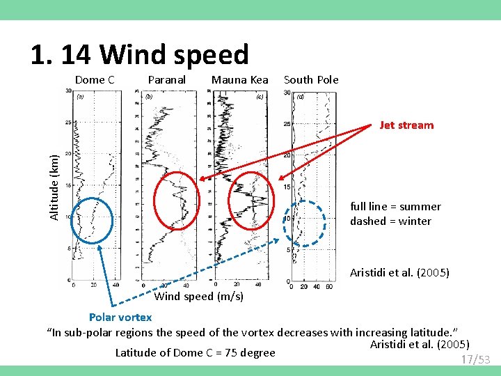
1. 14 Wind speed Dome C Paranal Mauna Kea South Pole Altitude (km) Jet stream full line = summer dashed = winter Aristidi et al. (2005) Wind speed (m/s) Polar vortex “In sub-polar regions the speed of the vortex decreases with increasing latitude. ” Aristidi et al. (2005) Latitude of Dome C = 75 degree 17/53

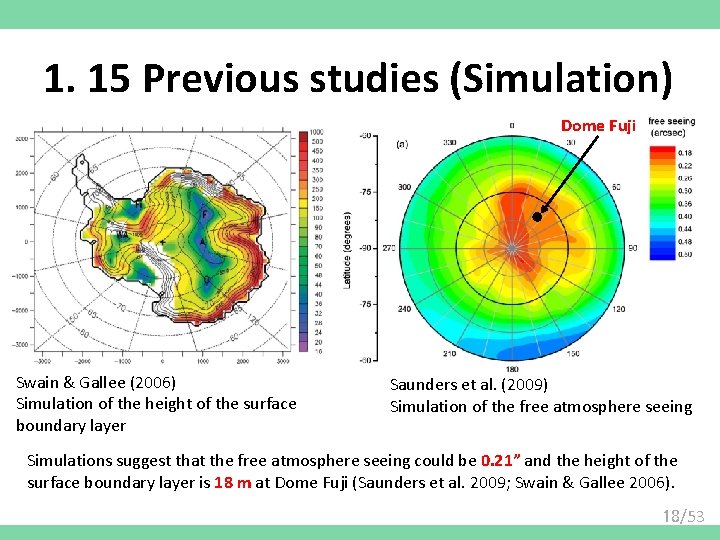
1. 15 Previous studies (Simulation) Dome Fuji Swain & Gallee (2006) Simulation of the height of the surface boundary layer Saunders et al. (2009) Simulation of the free atmosphere seeing Simulations suggest that the free atmosphere seeing could be 0. 21” and the height of the surface boundary layer is 18 m at Dome Fuji (Saunders et al. 2009; Swain & Gallee 2006). 18/53

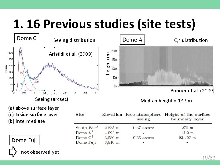
1. 16 Previous studies (site tests) Dome A Seeing distribution Aristidi et al. (2009) CT 2 distribution height (m) Dome C Bonner et al. (2009) Seeing (arcsec) Median height = 13. 9 m (a) above surface layer (c) Inside surface layer (b) intermediate Dome Fuji not observed yet 19/53

1. 17 Aim of this study The aim of this study is to investigate the astronomical seeing in the free atmosphere above and to determine the height of the surface boundary layer at Dome Fuji on the Antarctic plateau. 20/53

Contents 1. Introduction 2. Instrumentations 3. Data processing and error analysis 4. Results 5. Discussion and conclusion 6. Future work 21/53

2. 1 Measuring quantity Refractive index structure function Phase structure function Fried parameter Seeing 22/53

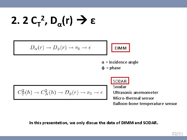
2, 2. 2 CT Dα(r) ε DIMM α = incidence angle φ = phase SODAR Snodar Ultrasonic anemometer Micro-thermal sensor Balloon-bone temperature sensor In this presentation, we only discus the data of DIMM and SODAR. 23/53

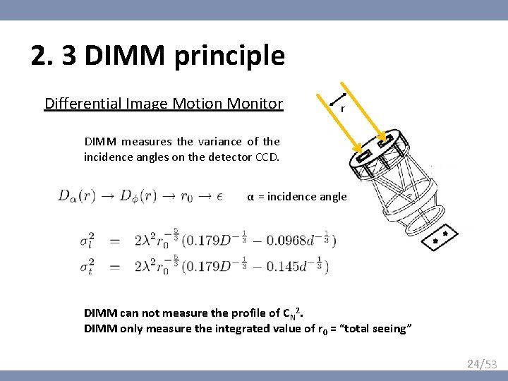
2. 3 DIMM principle Differential Image Motion Monitor r DIMM measures the variance of the incidence angles on the detector CCD. α = incidence angle DIMM can not measure the profile of CN 2. DIMM only measure the integrated value of r 0 = “total seeing” 24/53

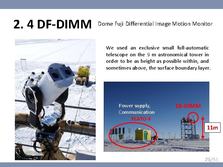
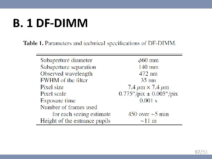
2. 4 DF-DIMM Dome Fuji Differential Image Motion Monitor We used an exclusive small full-automatic telescope on the 9 m astronomical tower in order to be as height as possible within, and sometimes above, the surface boundary layer. Power supply, Communication PLATO-F DF-DIMM 11 m 25/53

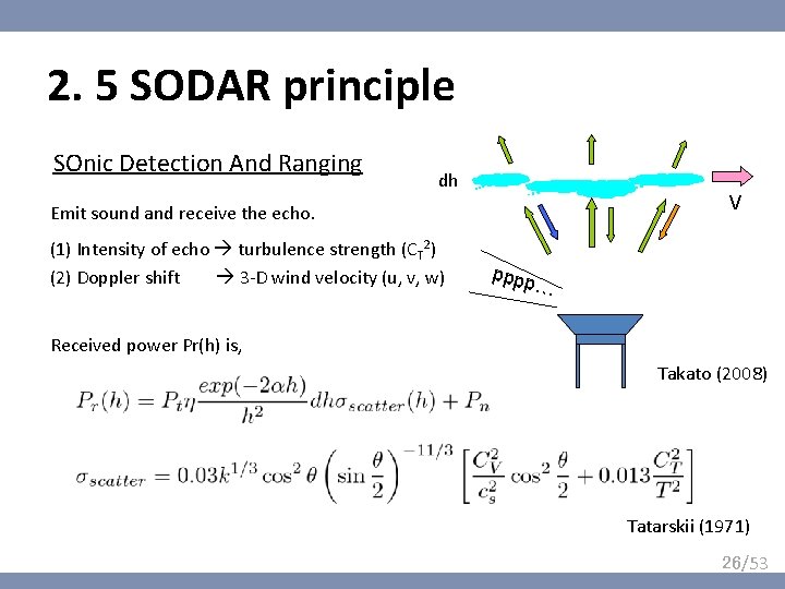
2. 5 SODAR principle SOnic Detection And Ranging dh V Emit sound and receive the echo. (1) Intensity of echo turbulence strength (CT 2) (2) Doppler shift 3 -D wind velocity (u, v, w) pppp … Received power Pr(h) is, Takato (2008) Tatarskii (1971) 26/53

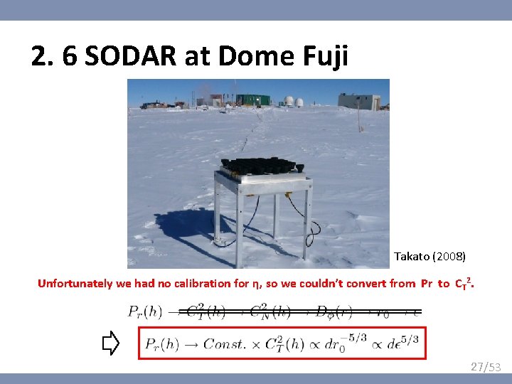
2. 6 SODAR at Dome Fuji Takato (2008) Unfortunately we had no calibration for η, so we couldn’t convert from Pr to CT 2. 27/53

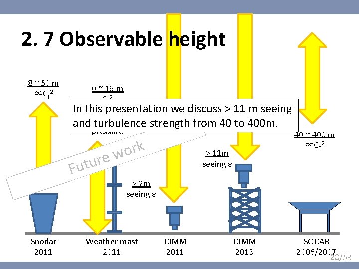
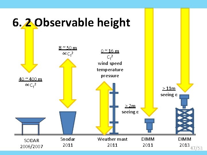
2. 7 Observable height 8 ~ 50 m ∝CT 2 0 ~ 16 m CT 2 In this we discuss > 11 m seeing wind presentation speed temperature and turbulence strength from 40 to 400 m. pressure 40 ~ 400 m k r o re w Futu Snodar 2011 ∝CT 2 > 11 m seeing ε > 2 m seeing ε Weather mast 2011 DIMM 2013 SODAR 2006/2007 28/53

Contents 1. Introduction 2. Instrumentations 3. Data processing and error analysis 4. Results 5. Discussion and conclusion 6. Future work 29/53

Contents 1. Introduction 2. Instrumentations 3. Data processing and error analysis 4. Results 5. Discussion and conclusion 6. Future work 30/53

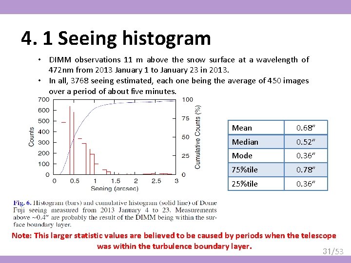
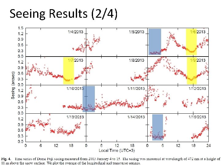
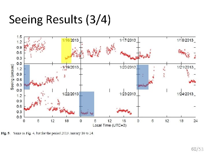
4. 1 Seeing histogram • DIMM observations 11 m above the snow surface at a wavelength of 472 nm from 2013 January 1 to January 23 in 2013. • In all, 3768 seeing estimated, each one being the average of 450 images over a period of about five minutes. Mean 0. 68” Median 0. 52” Mode 0. 36” 75%tile 0. 78” 25%tile 0. 36” Note: This larger statistic values are believed to be caused by periods when the telescope was within the turbulence boundary layer. 31/53

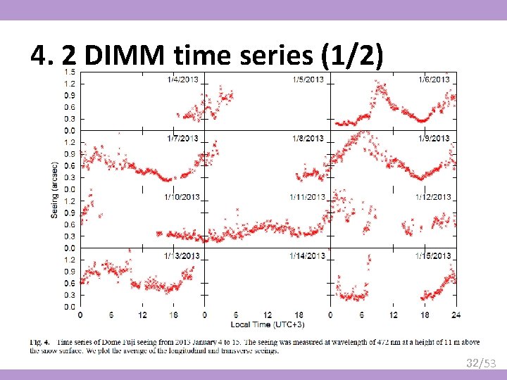
4. 2 DIMM time series (1/2) 32/53

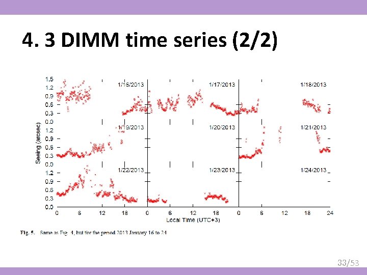
4. 3 DIMM time series (2/2) 33/53

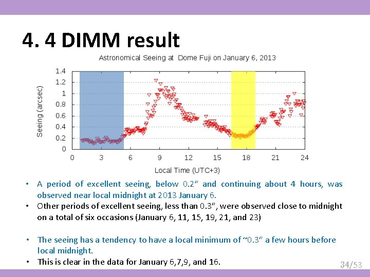
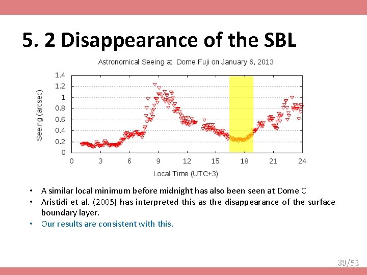
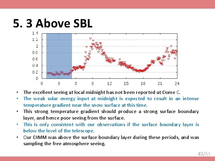
4. 4 DIMM result • A period of excellent seeing, below 0. 2” and continuing about 4 hours, was observed near local midnight at 2013 January 6. • Other periods of excellent seeing, less than 0. 3”, were observed close to midnight on a total of six occasions (January 6, 11, 15, 19, 21, and 23) • The seeing has a tendency to have a local minimum of ~0. 3” a few hours before local midnight. • This is clear in the data for January 6, 7, 9, and 16. 34/53

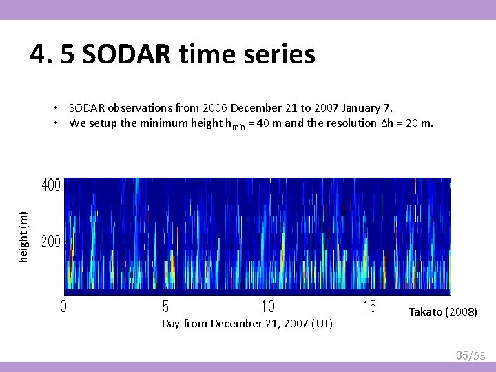
4. 5 SODAR time series height (m) • SODAR observations from 2006 December 21 to 2007 January 7. • We setup the minimum height hmin = 40 m and the resolution Δh = 20 m. Day from December 21, 2007 (UT) Takato (2008) 35/53

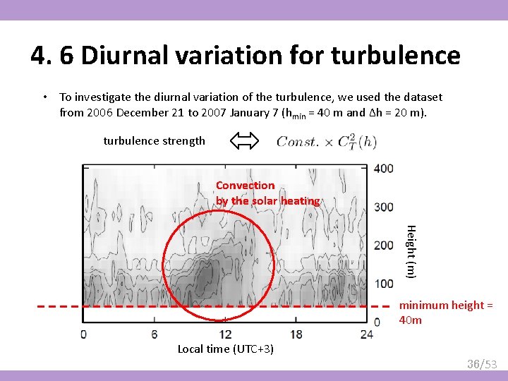
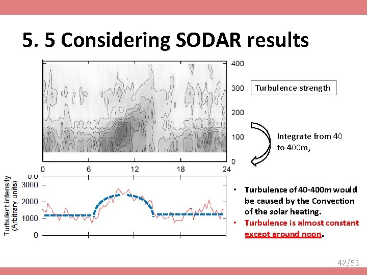
4. 6 Diurnal variation for turbulence • To investigate the diurnal variation of the turbulence, we used the dataset from 2006 December 21 to 2007 January 7 (hmin = 40 m and Δh = 20 m). turbulence strength Convection by the solar heating Height (m) minimum height = 40 m Local time (UTC+3) 36/53

Contents 1. Introduction 2. Instrumentations 3. Data processing and error analysis 4. Results 5. Discussion and conclusion 6. Future work 37/53

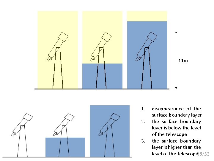
5. 1 Cause for excellent seeing Height ~10 km Model of the atmosphere structure at “Dome” on the Antarctic plateau Stratosphere Troposphere Free Atmosphere 10 ~ 200 m Surface Boundary Layer 1) 2) 3) 1. 2. 3. disappearance of the surface boundary layer is below the level of the telescope the surface boundary layer is higher than the level of the telescope 38/53

5. 2 Disappearance of the SBL • A similar local minimum before midnight has also been seen at Dome C • Aristidi et al. (2005) has interpreted this as the disappearance of the surface boundary layer. • Our results are consistent with this. 39/53

5. 3 Above SBL • The excellent seeing at local midnight has not been reported at Dome C. • The weak solar energy input at midnight is expected to result in an intense temperature gradient near the snow surface at this time. • This strong temperature gradient should produce a strong surface boundary layer, and hence poor seeing from the surface. • This is only consistent with our observations if the surface boundary layer is below the level of the telescope. • Our DIMM was above the surface boundary layer during these periods, and was sampling the free atmosphere seeing. 40/53

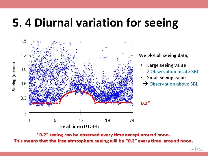
5. 4 Diurnal variation for seeing We plot all seeing data, • Large seeing value Observation inside SBL • Small seeing value Observation above SBL 0. 2” 0 6 12 Local time (UTC+3) 18 24 ~0. 2” seeing can be observed every time except around noon. This means that the free atmosphere seeing will be ~0. 2” every time around noon. 41/53

5. 5 Considering SODAR results Turbulence strength Integrate from 40 to 400 m, • Turbulence of 40 -400 m would be caused by the Convection of the solar heating. • Turbulence is almost constant except around noon. 42/53

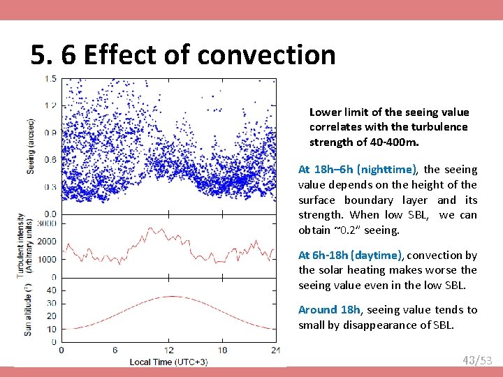
5. 6 Effect of convection Lower limit of the seeing value correlates with the turbulence strength of 40 -400 m. At 18 h– 6 h (nighttime), the seeing value depends on the height of the surface boundary layer and its strength. When low SBL, we can obtain ~0. 2” seeing. At 6 h-18 h (daytime), convection by the solar heating makes worse the seeing value even in the low SBL. Around 18 h, seeing value tends to small by disappearance of SBL. 43/53

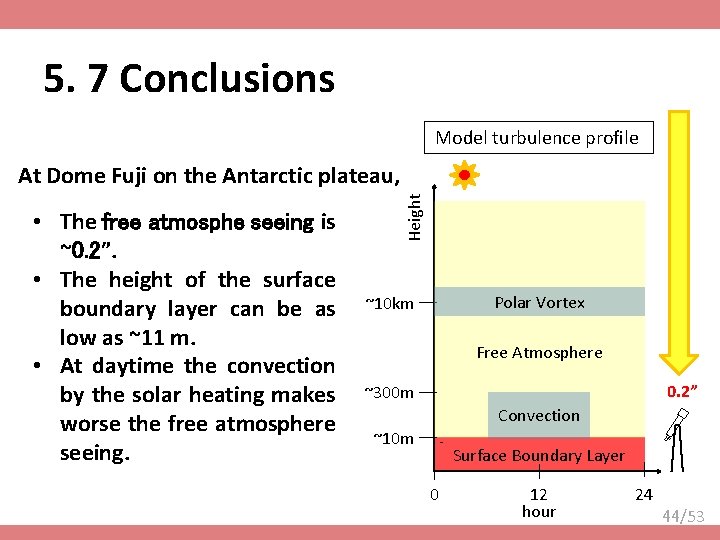
5. 7 Conclusions Model turbulence profile • The free atmosphe seeing is ~0. 2”. • The height of the surface boundary layer can be as low as ~11 m. • At daytime the convection by the solar heating makes worse the free atmosphere seeing. Height At Dome Fuji on the Antarctic plateau, Polar Vortex ~10 km Free Atmosphere 0. 2” ~300 m Convection ~10 m Surface Boundary Layer 0 12 hour 24 44/53

Contents 1. Introduction 2. Instrumentations 3. Data processing and error analysis 4. Results 5. Discussion and conclusion 6. Future work 45/53

6. 1 Aim of this study The aim of this study is to investigate the astronomical seeing in the free atmosphere above and to determine the height of the surface boundary layer at Dome Fuji on the Antarctic plateau. 46/53

6. 2 Observable height 8 ~ 50 m ∝CT 2 40 ~ 400 m ∝CT 2 0 ~ 16 m CT 2 wind speed temperature pressure > 11 m seeing ε > 2 m seeing ε SODAR 2006/2007 Snodar 2011 Weather mast 2011 DIMM 2013 47/53

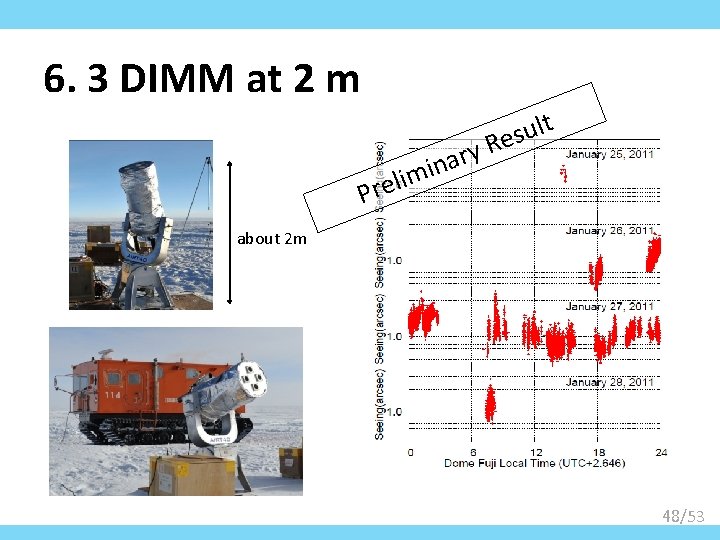
6. 3 DIMM at 2 m y r a n i m i l Pre lt u s Re about 2 m 48/53

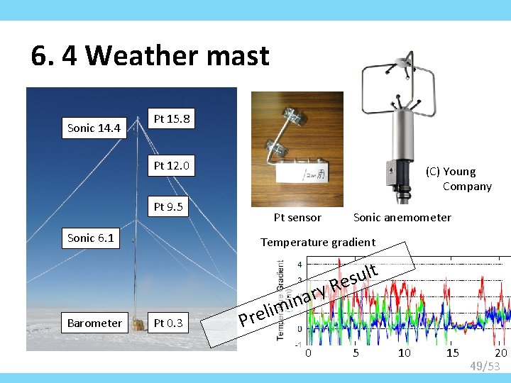
6. 4 Weather mast Sonic 14. 4 Pt 15. 8 Pt 12. 0 Pt 9. 5 Sonic 6. 1 Barometer (C) Young Company Pt sensor Sonic anemometer Temperature gradient Pt 0. 3 m i l e Pr y r a in 0 lt u s Re 5 10 15 20 49/53

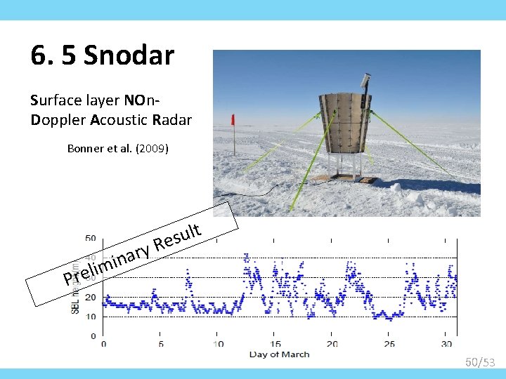
6. 5 Snodar Surface layer NOn. Doppler Acoustic Radar Bonner et al. (2009) y r a n imi lt u s Re l e r P 50/53

6. 6 Aim of this study The aim of this study is to investigate the astronomical seeing in the free atmosphere above and to determine the height of the surface boundary layer at Dome Fuji on the Antarctic plateau. Future Work 51/53

Acknowledgements We acknowledge the National Institute of Polar Research and the 51 st - 54 th Japanese Antarctic Research Expeditions. This research is supported by the National Institute of Polar Research through Project Research no. KP-12, the Grants-in. Aid for Scientific Research 18340050 and 23103002, the Australian Research Council and Australian government infrastructure funding managed by Astronomy Australia Limited. Hirofumi Okita thanks the Sasakawa Scientific Research Grant from The Japan Science Society, and Tohoku University International Advanced Research and Education Organization for scholarships and research expenses. 52/53

Thank you. 53/53

Contents 1. Introduction 2. Instrumentations 3. Data processing and error analysis 4. Results 5. Discussion and conclusion 6. Future work 7. Appendix 54/53

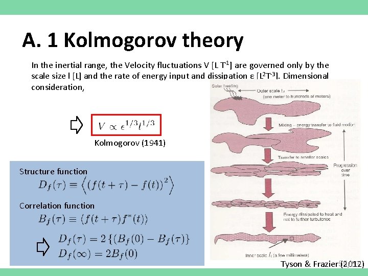
A. 1 Kolmogorov theory In the inertial range, the Velocity fluctuations V [L T-1] are governed only by the scale size l [L] and the rate of energy input and dissipation ε [L 2 T-3]. Dimensional consideration, Kolmogorov (1941) Structure function Correlation function Tyson & Frazier 55/53 (2012)

A. 2 Structure function Velocity structure function Tatarskii (1971) Temperature structure function Refractivity P = pressure in mill bar T = temperature, K Refractive index structure function 56/53

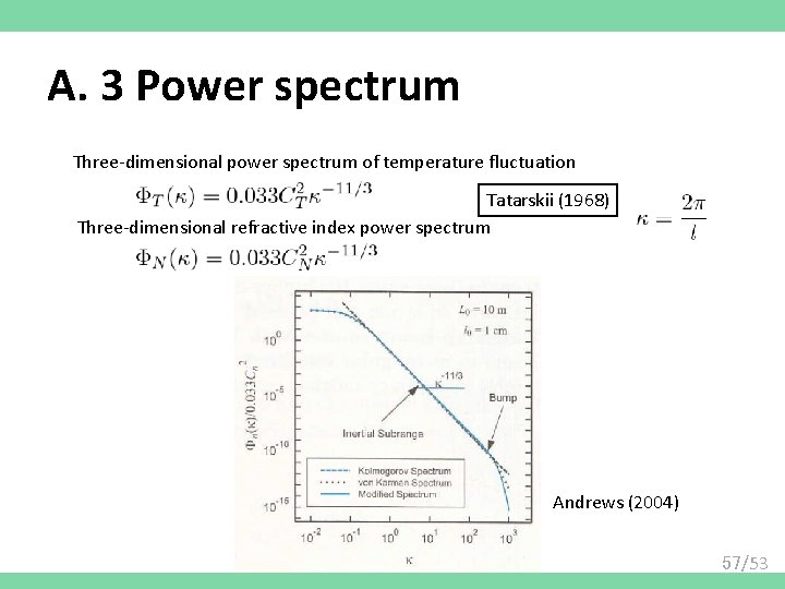
A. 3 Power spectrum Three-dimensional power spectrum of temperature fluctuation Tatarskii (1968) Three-dimensional refractive index power spectrum Andrews (2004) 57/53

A. 4 Phase structure function Phase shift Phase correlation function Phase structure function 58/53

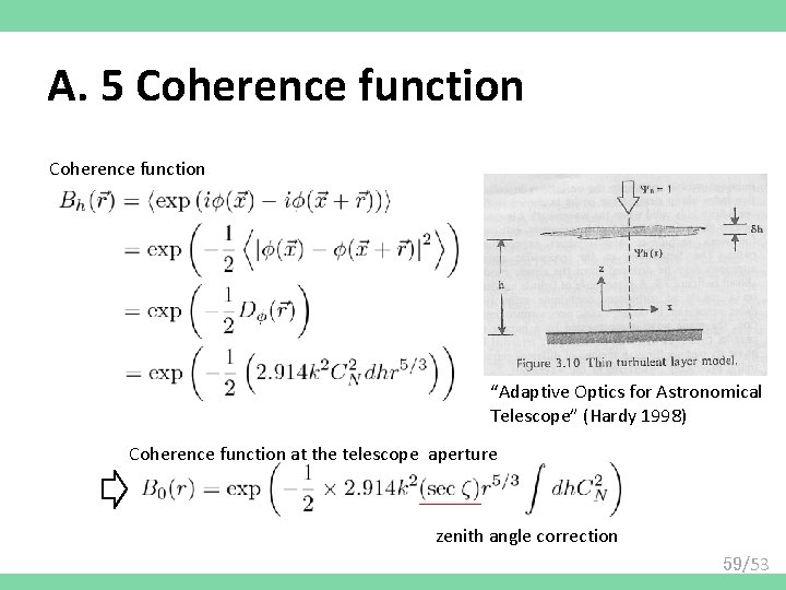
A. 5 Coherence function “Adaptive Optics for Astronomical Telescope” (Hardy 1998) Coherence function at the telescope aperture zenith angle correction 59/53

A. 6 Optical transfer function B(f) = atmospheric transfer function T(f) = telescope transfer function Small aperture Large aperture Fried also defined the parameter r 0, which is the diameter of a telescope which would have the same resolving power as the atmospheric transfer function 60/53

A. 7 Fried parameter Here, B(f) may be written Fried parameter Phase structure function 61/53

B. 1 DF-DIMM 62/53

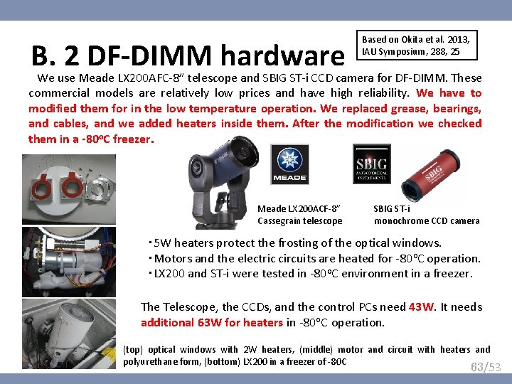
B. 2 DF-DIMM hardware Based on Okita et al. 2013, IAU Symposium, 288, 25 We use Meade LX 200 AFC-8” telescope and SBIG ST-i CCD camera for DF-DIMM. These commercial models are relatively low prices and have high reliability. We have to modified them for in the low temperature operation. We replaced grease, bearings, and cables, and we added heaters inside them. After the modification we checked them in a -80 o. C freezer. Meade LX 200 ACF-8” Cassegrain telescope SBIG ST-i monochrome CCD camera ・ 5 W heaters protect the frosting of the optical windows. ・Motors and the electric circuits are heated for -80 o. C operation. ・LX 200 and ST-i were tested in -80 o. C environment in a freezer. The Telescope, the CCDs, and the control PCs need 43 W. It needs additional 63 W for heaters in -80 o. C operation. (top) optical windows with 2 W heaters, (middle) motor and circuit with heaters and polyurethane form, (bottom) LX 200 in a freezer of -80 C 63/53

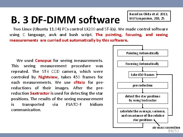
B. 3 DF-DIMM software Based on Okita et al. 2013, IAU Symposium, 288, 25 Two Linux (Ubuntu 11. 04) PCs control LX 200 and ST-i(s). We made control software using C language, awk and bash script. The pointing, focusing, and seeing measurements are curried out automatically by this software. Pointing Automatically We used Canopus for seeing measurements. This seeing measurement procedure was repeated. The ST-i CCD camera, which were controled by Nightview, takes 450 frames for each measurements. We use cfitsio for prereductions of their images. After the prereduction Sextractor is used for detecting the star positions. The results of the seeing measurement is transported via PLATO-F Iridium communication. Focusing Automatically take 450 frames pre-reduction detect the star positions by using Sextractor calculate the average, variance, and covariance of the relative star positions air-mass correction 64/53

65/53

11 m 1. 2. 3. disappearance of the surface boundary layer is below the level of the telescope the surface boundary layer is higher than the level of the telescope 66/53

Seeing Results (2/4) 67/53

Seeing Results (3/4) 68/53