ASSUMPTION CHECKING In regression analysis with Stata In

ASSUMPTION CHECKING • In regression analysis with Stata • In multi-level analysis with Stata (not much extra) • In logistic regression analysis with Stata NOTE: THIS WILL BE EASIER IN STATA THAN IT WAS IN SPSS

Assumption checking in “normal” multiple regression with Stata

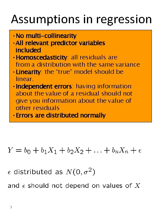
Assumptions in regression • No multi-collinearity analysis • All relevant predictor variables included • Homoscedasticity: all residuals are from a distribution with the same variance • Linearity: the “true” model should be linear. • Independent errors: having information about the value of a residual should not give you information about the value of other residuals • Errors are distributed normally 3

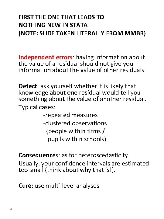
FIRST THE ONE THAT LEADS TO NOTHING NEW IN STATA (NOTE: SLIDE TAKEN LITERALLY FROM MMBR) Independent errors: having information about the value of a residual should not give you information about the value of other residuals Detect: ask yourself whether it is likely that knowledge about one residual would tell you something about the value of another residual. Typical cases: -repeated measures -clustered observations (people within firms / pupils within schools) Consequences: as for heteroscedasticity Usually, your confidence intervals are estimated too small (think about why that is!). Cure: use multi-level analyses 4

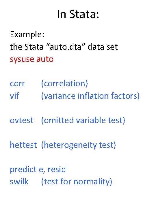
In Stata: Example: the Stata “auto. dta” data set sysuse auto corr vif (correlation) (variance inflation factors) ovtest (omitted variable test) hettest (heterogeneity test) predict e, resid swilk (test for normality)

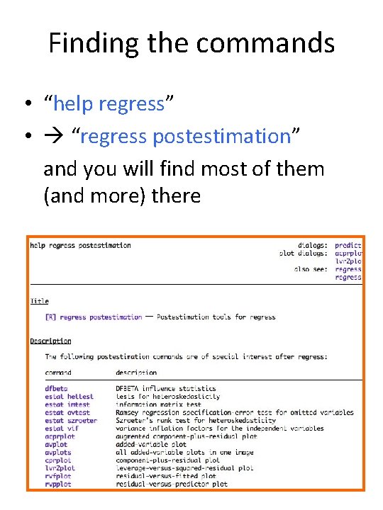
Finding the commands • “help regress” • “regress postestimation” and you will find most of them (and more) there

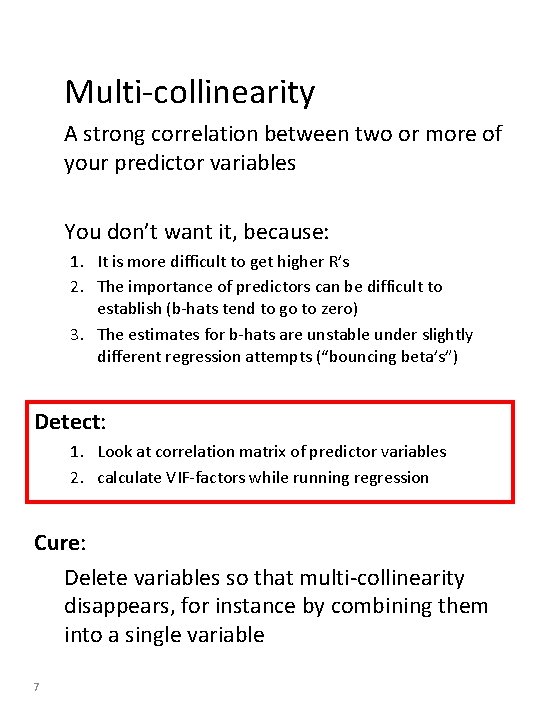
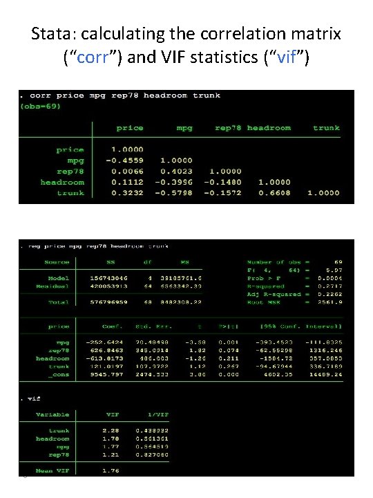
Multi-collinearity A strong correlation between two or more of your predictor variables You don’t want it, because: 1. It is more difficult to get higher R’s 2. The importance of predictors can be difficult to establish (b-hats tend to go to zero) 3. The estimates for b-hats are unstable under slightly different regression attempts (“bouncing beta’s”) Detect: 1. Look at correlation matrix of predictor variables 2. calculate VIF-factors while running regression Cure: Delete variables so that multi-collinearity disappears, for instance by combining them into a single variable 7

Stata: calculating the correlation matrix (“corr”) and VIF statistics (“vif”) 8

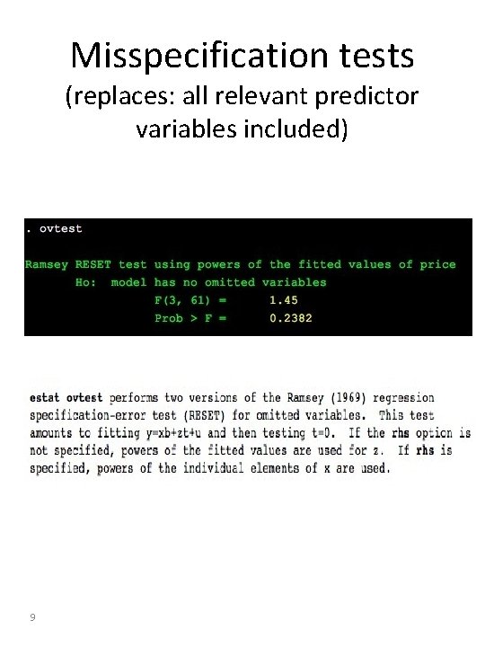
Misspecification tests (replaces: all relevant predictor variables included) 9

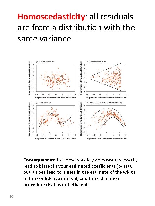
Homoscedasticity: all residuals are from a distribution with the same variance Consequences: Heteroscedasticiy does not necessarily lead to biases in your estimated coefficients (b-hat), but it does lead to biases in the estimate of the width of the confidence interval, and the estimation procedure itself is not efficient. 10

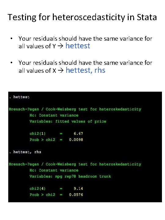
Testing for heteroscedasticity in Stata • Your residuals should have the same variance for all values of Y hettest • Your residuals should have the same variance for all values of X hettest, rhs

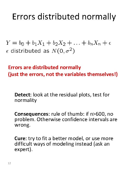
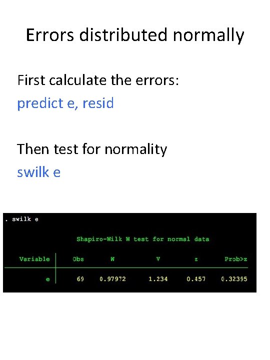
Errors distributed normally Errors are distributed normally (just the errors, not the variables themselves!) Detect: look at the residual plots, test for normality Consequences: rule of thumb: if n>600, no problem. Otherwise confidence intervals are wrong. Cure: try to fit a better model, or use more difficult ways of modeling instead (ask an expert). 12

Errors distributed normally First calculate the errors: predict e, resid Then test for normality swilk e

Assumption checking in multi-level multiple regression with Stata

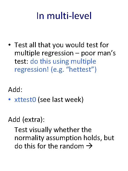
In multi-level • Test all that you would test for multiple regression – poor man’s test: do this using multiple regression! (e. g. “hettest”) Add: • xttest 0 (see last week) Add (extra): Test visually whether the normality assumption holds, but do this for the random

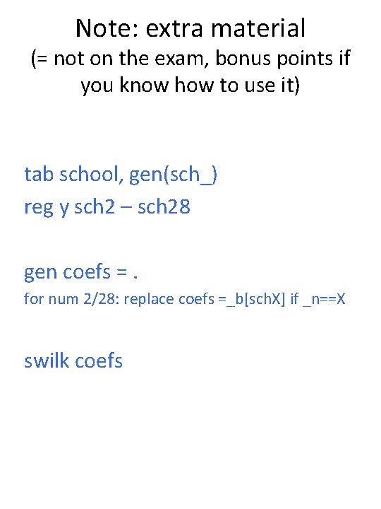
Note: extra material (= not on the exam, bonus points if you know how to use it) tab school, gen(sch_) reg y sch 2 – sch 28 gen coefs =. for num 2/28: replace coefs =_b[sch. X] if _n==X swilk coefs

Assumption checking in multi-level multiple regression with Stata

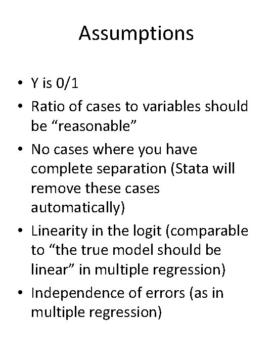
Assumptions • Y is 0/1 • Ratio of cases to variables should be “reasonable” • No cases where you have complete separation (Stata will remove these cases automatically) • Linearity in the logit (comparable to “the true model should be linear” in multiple regression) • Independence of errors (as in multiple regression)

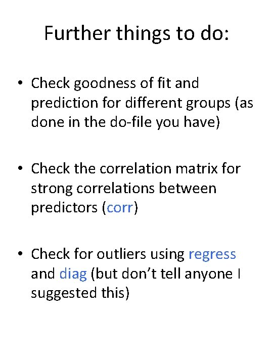
Further things to do: • Check goodness of fit and prediction for different groups (as done in the do-file you have) • Check the correlation matrix for strong correlations between predictors (corr) • Check for outliers using regress and diag (but don’t tell anyone I suggested this)