Association Rules Correlations z Basic concepts z Efficient
Association Rules & Correlations z Basic concepts z Efficient and scalable frequent itemset mining methods: y Apriori, and improvements y FP-growth z Rule postmining: visualization and validation z Interesting association rules. 1
Rule Validations z Only a small subset of derived rules might be meaningful/useful y. Domain expert must validate the rules z Useful tools: y. Visualization y. Correlation analysis 2
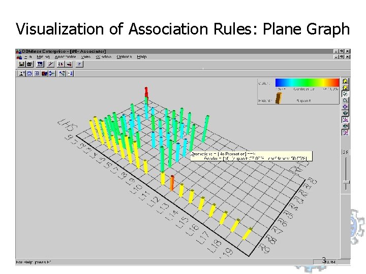
Visualization of Association Rules: Plane Graph 3
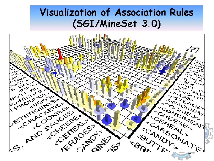
Visualization of Association Rules (SGI/Mine. Set 3. 0) 4
Pattern Evaluation z. Association rule algorithms tend to produce too many rules y many of them are uninteresting or redundant y confidence(A B) = p(B|A) = p(A & B)/p(A) y Confidence is not discriminative enough criterion y Beyond original support & confidence y Interestingness measures can be used to prune/rank the derived patterns 5
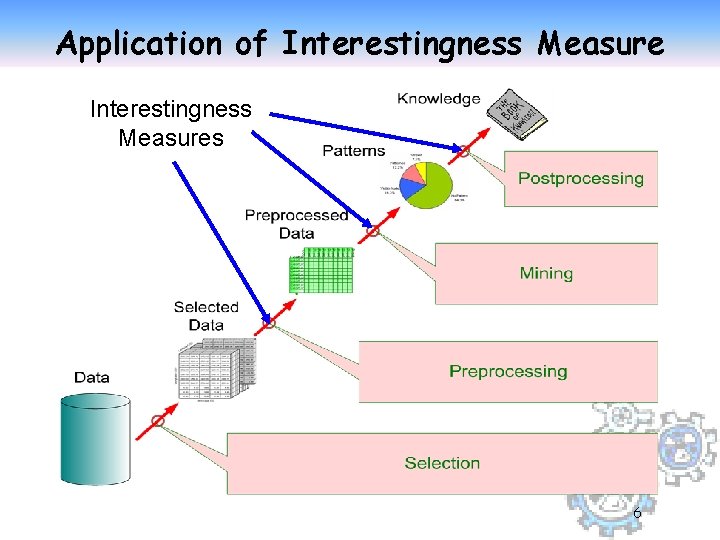
Application of Interestingness Measures 6
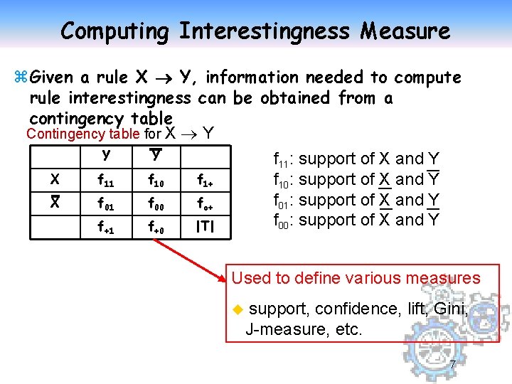
Computing Interestingness Measure z. Given a rule X Y, information needed to compute rule interestingness can be obtained from a contingency table Contingency table for X Y Y Y f 11: support of X and Y X f 11 f 10 f 1+ f 10: support of X and Y f 01: support of X and Y X f 01 f 00 fo+ f 00: support of X and Y f+1 f+0 |T| Used to define various measures u support, confidence, lift, Gini, J-measure, etc. 7
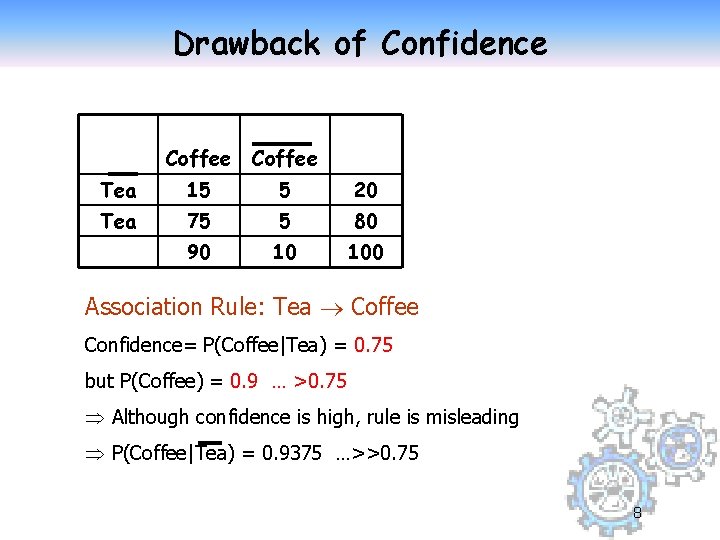
Drawback of Confidence Coffee Tea 15 5 20 Tea 75 5 80 90 10 100 Association Rule: Tea Coffee Confidence= P(Coffee|Tea) = 0. 75 but P(Coffee) = 0. 9 … >0. 75 Although confidence is high, rule is misleading P(Coffee|Tea) = 0. 9375 …>>0. 75 8
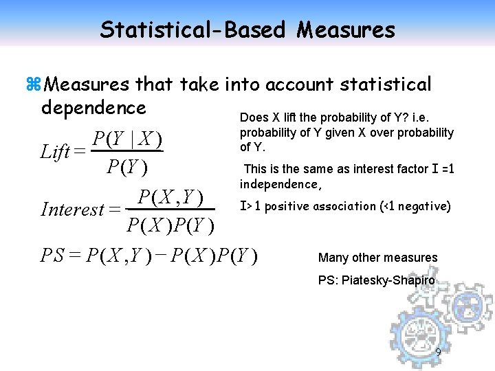
Statistical-Based Measures z. Measures that take into account statistical dependence Does X lift the probability of Y? i. e. probability of Y given X over probability P(Y | X ) of Y. Lift = This is the same as interest factor I =1 P(Y ) independence, P( X , Y ) I> 1 positive association (<1 negative) = Interest P( X ) P(Y ) PS = P( X , Y ) - P( X ) P(Y ) Many other measures PS: Piatesky-Shapiro 9
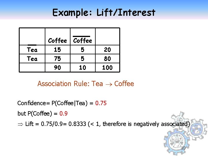
Example: Lift/Interest Coffee Tea 15 5 20 Tea 75 5 80 90 10 100 Association Rule: Tea Coffee Confidence= P(Coffee|Tea) = 0. 75 but P(Coffee) = 0. 9 Lift = 0. 75/0. 9= 0. 8333 (< 1, therefore is negatively associated) 10
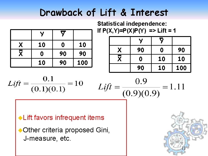
Drawback of Lift & Interest Statistical independence: If P(X, Y)=P(X)P(Y) => Lift = 1 Y Y X 10 0 10 X 0 90 90 100 u. Lift Y Y X 90 0 90 X 0 10 10 90 10 100 favors infrequent items u. Other criteria proposed Gini, J-measure, etc. 11
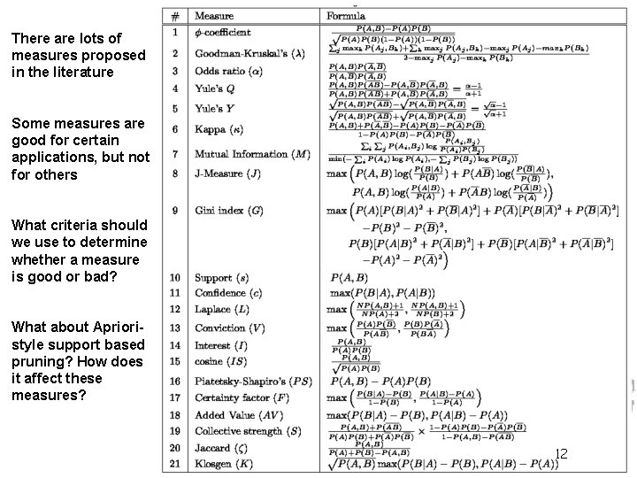
There are lots of measures proposed in the literature Some measures are good for certain applications, but not for others What criteria should we use to determine whether a measure is good or bad? What about Aprioristyle support based pruning? How does it affect these measures? 12

Association Rules & Correlations z Basic concepts z Efficient and scalable frequent itemset mining methods: y Apriori, and improvements y FP-growth z Rule derivation, visualization and validation z Multi-level Associations z Summary 13
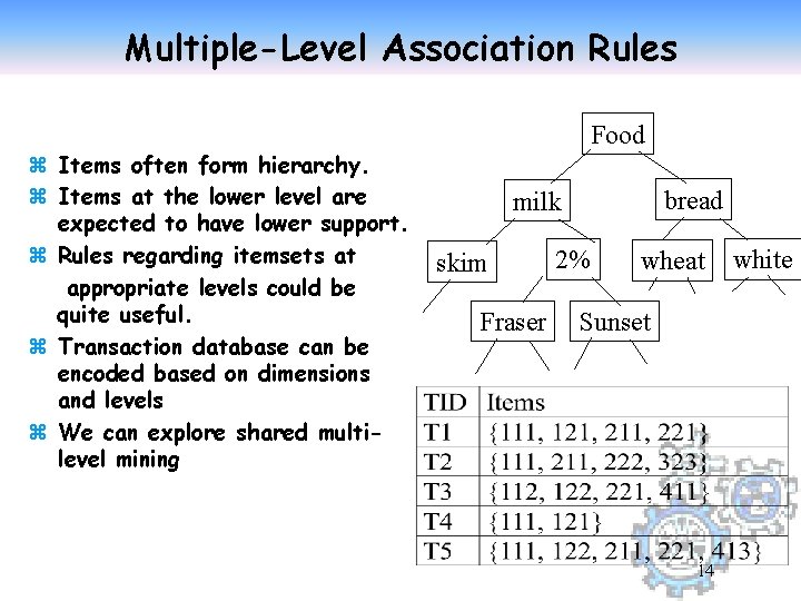
Multiple-Level Association Rules z Items often form hierarchy. z Items at the lower level are expected to have lower support. z Rules regarding itemsets at appropriate levels could be quite useful. z Transaction database can be encoded based on dimensions and levels z We can explore shared multilevel mining Food bread milk skim Fraser 2% wheat Sunset 14 white
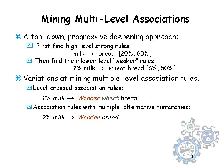
Mining Multi-Level Associations z A top_down, progressive deepening approach: y First find high-level strong rules: milk ® bread [20%, 60%]. y Then find their lower-level “weaker” rules: 2% milk ® wheat bread [6%, 50%]. z Variations at mining multiple-level association rules. y Level-crossed association rules: 2% milk ® Wonder wheat bread y Association rules with multiple, alternative hierarchies: 2% milk ® Wonder bread 15
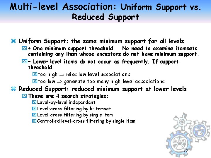
Multi-level Association: Uniform Support vs. Reduced Support z Uniform Support: the same minimum support for all levels y + One minimum support threshold. No need to examine itemsets containing any item whose ancestors do not have minimum support. y – Lower level items do not occur as frequently. If support threshold xtoo high miss low level associations xtoo low generate too many high level associations z Reduced Support: reduced minimum support at lower levels y There are 4 search strategies: x Level-by-level independent x Level-cross filtering by k-itemset x Level-cross filtering by single item x Controlled level-cross filtering by single item 16
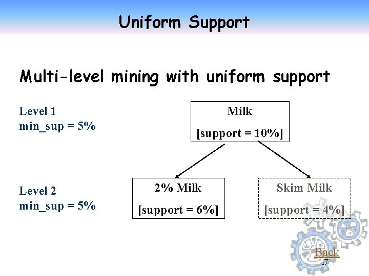
Uniform Support Multi-level mining with uniform support Level 1 min_sup = 5% Level 2 min_sup = 5% Milk [support = 10%] 2% Milk Skim Milk [support = 6%] [support = 4%] Back 17
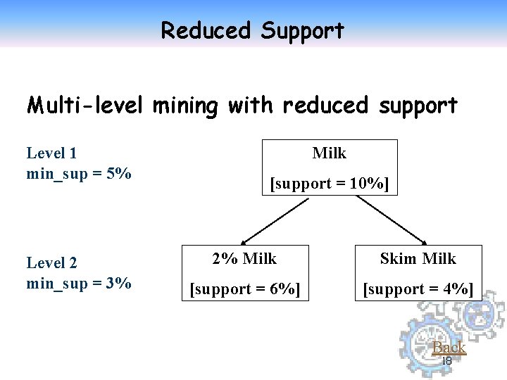
Reduced Support Multi-level mining with reduced support Level 1 min_sup = 5% Level 2 min_sup = 3% Milk [support = 10%] 2% Milk Skim Milk [support = 6%] [support = 4%] Back 18
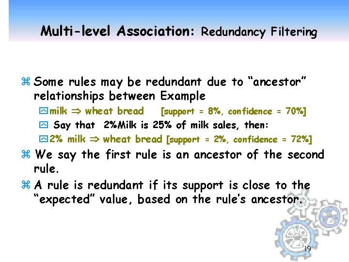
Multi-level Association: Redundancy Filtering z Some rules may be redundant due to “ancestor” relationships between Example y milk wheat bread [support = 8%, confidence = 70%] y Say that 2%Milk is 25% of milk sales, then: y 2% milk wheat bread [support = 2%, confidence = 72%] z We say the first rule is an ancestor of the second rule. z A rule is redundant if its support is close to the “expected” value, based on the rule’s ancestor. 19
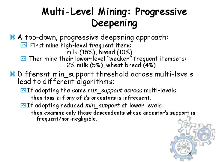
Multi-Level Mining: Progressive Deepening z A top-down, progressive deepening approach: y First mine high-level frequent items: milk (15%), bread (10%) y Then mine their lower-level “weaker” frequent itemsets: 2% milk (5%), wheat bread (4%) z Different min_support threshold across multi-levels lead to different algorithms: y If adopting the same min_support across multi-levels then toss t if any of t’s ancestors is infrequent. y If adopting reduced min_support at lower levels then examine only those descendents whose ancestor’s support is frequent/non-negligible. 20
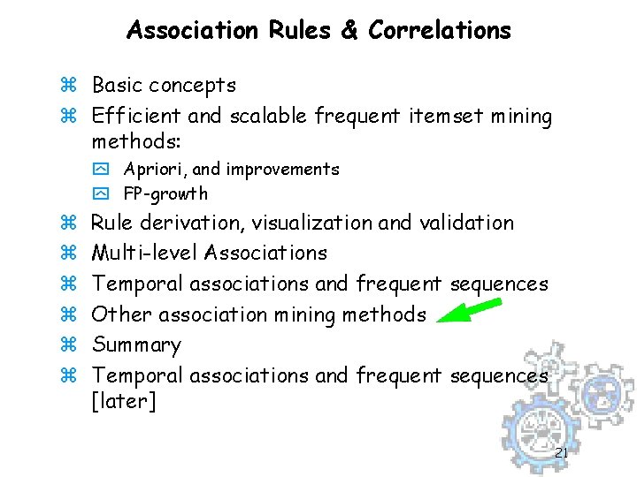
Association Rules & Correlations z Basic concepts z Efficient and scalable frequent itemset mining methods: y Apriori, and improvements y FP-growth z z z Rule derivation, visualization and validation Multi-level Associations Temporal associations and frequent sequences Other association mining methods Summary Temporal associations and frequent sequences [later] 21
Other Association Mining Methods z z z z CHARM: Mining frequent itemsets by a Vertical Data Format Mining Frequent Closed Patterns Mining Max-patterns Mining Quantitative Associations [e. g. , what is the implication between age and income? ] Constraint-base association mining Frequent Patterns in Data Streams: very difficult problem. Performance is a real issue Constraint-based (Query-Directed) Mining sequential and structured patterns 22
Summary z Association rule mining yprobably the most significant contribution from the database community in KDD z New interesting research directions y. Association analysis in other types of data: spatial data, multimedia data, time series data, z Association Rule Mining for Data Streams: a very difficult challenge. 23
Statistical Independence z. Population of 1000 students y 600 students know how to swim (S) y 700 students know how to bike (B) y 420 students know how to swim and bike (S, B) y P(S B) = 420/1000 = 0. 42 y P(S) P(B) = 0. 6 0. 7 = 0. 42 y P(S B) = P(S) P(B) => Statistical independence y P(S B) > P(S) P(B) => Positively correlated 24 y P(S B) < P(S) P(B) => Negatively correlated
- Slides: 24