Association does not imply causation Correlation Coefficient Simple

Association does not imply causation Correlation Coefficient & Simple Linear Regression Correlation does not assume causality but regression does. STATS 101 Laurens Holmes, Jr.

Sir Galton was the first to apply the word regression to biological and psychological data. Specifically, Galton observed the heights of children versus the heights of their parents. He discovered that taller than average parents tended to have children who were also taller than average, but not as tall as their parents. Galton characterized this as regression toward mediocrity. Correlation Coefficient is also attributed to Francis Galton. Regression implies “……. to go backward”, Why are statistical methods for predicting a response from an explanatory variable termed “regression”? SIR FRANCIS GALTON (1822 -1911)

Correlation r • Linear relationships implying straight line association are visualized with scatter plots • Strong linear relationship – When the points lie close to a straight line, and weak if they are widely scattered

Correlation r • Purpose: Measures the direction and strength of the linear relationship between two quantitative variables – Represented by r. – There is no assumption of causality – Assumes a linear association between two variables.

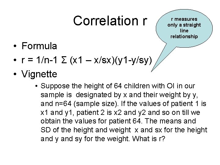
Correlation r r measures only a straight line relationship • Formula • r = 1/n-1 Σ (x 1 – x/sx)(y 1 -y/sy) • Vignette • Suppose the height of 64 children with OI in our sample is designated by x and their weight by y, and n=64 (sample size). If the values of patient 1 is x 1 and y 1, patient 2 is x 2 and y 2 and so on till we obtain the values for patient 64. The means and SD of the height and weight x and sx for the height and y and sy for the weight. What is r?

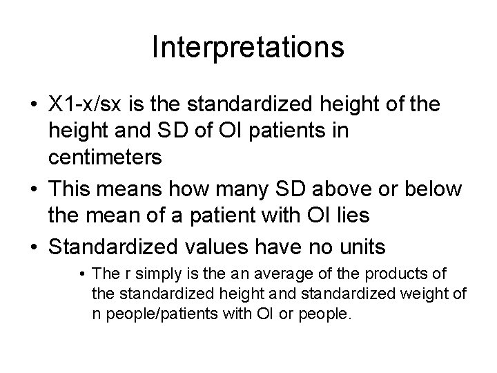
Interpretations • X 1 -x/sx is the standardized height of the height and SD of OI patients in centimeters • This means how many SD above or below the mean of a patient with OI lies • Standardized values have no units • The r simply is the an average of the products of the standardized height and standardized weight of n people/patients with OI or people.

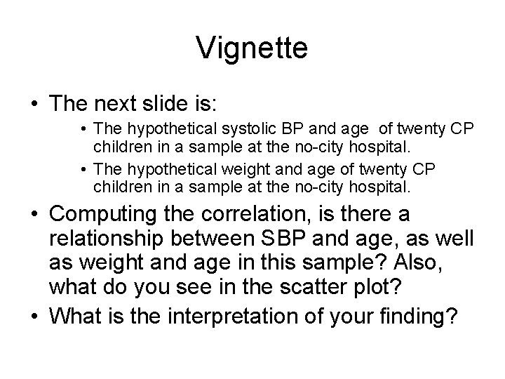
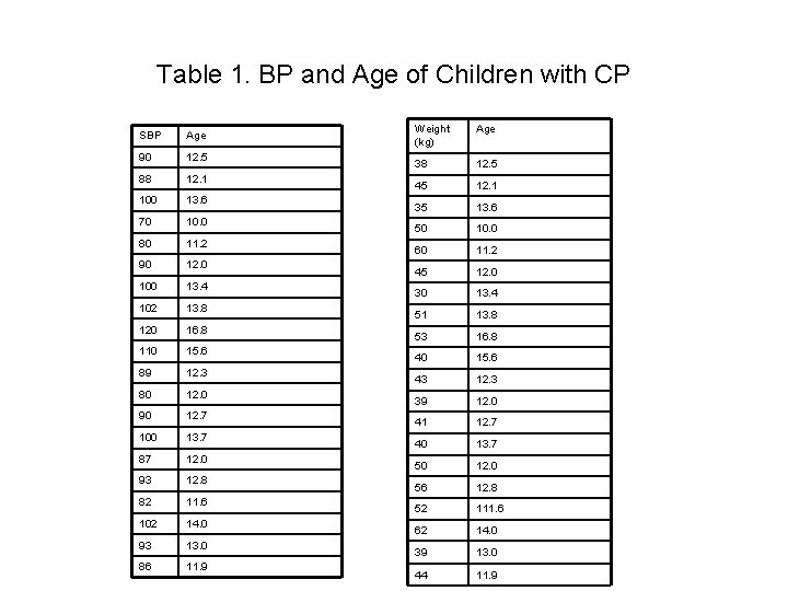
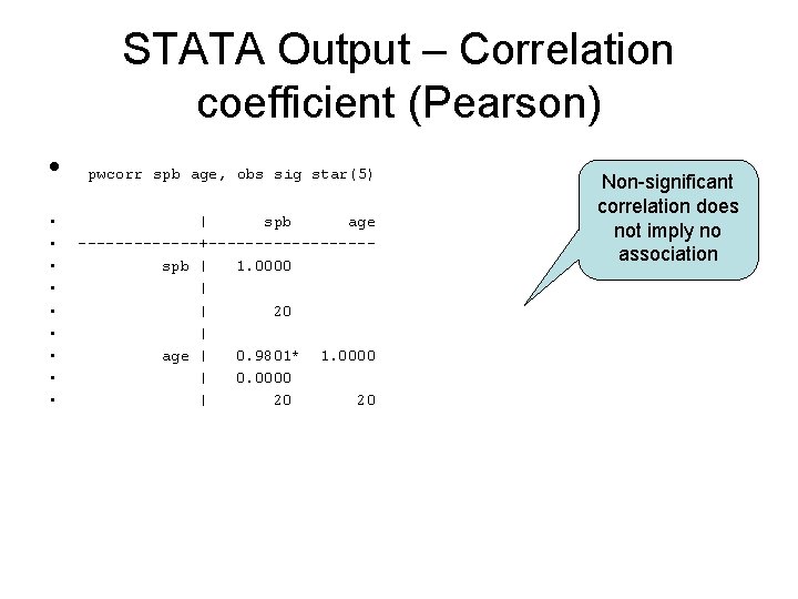
Vignette • The next slide is: • The hypothetical systolic BP and age of twenty CP children in a sample at the no-city hospital. • The hypothetical weight and age of twenty CP children in a sample at the no-city hospital. • Computing the correlation, is there a relationship between SBP and age, as well as weight and age in this sample? Also, what do you see in the scatter plot? • What is the interpretation of your finding?

Table 1. BP and Age of Children with CP SBP Age 90 12. 5 88 12. 1 100 13. 6 70 10. 0 80 11. 2 90 12. 0 100 13. 4 102 13. 8 120 16. 8 110 15. 6 89 12. 3 80 12. 0 90 12. 7 100 13. 7 87 12. 0 93 12. 8 82 11. 6 102 14. 0 93 13. 0 86 11. 9 Weight (kg) Age 38 12. 5 45 12. 1 35 13. 6 50 10. 0 60 11. 2 45 12. 0 30 13. 4 51 13. 8 53 16. 8 40 15. 6 43 12. 3 39 12. 0 41 12. 7 40 13. 7 50 12. 0 56 12. 8 52 111. 6 62 14. 0 39 13. 0 44 11. 9

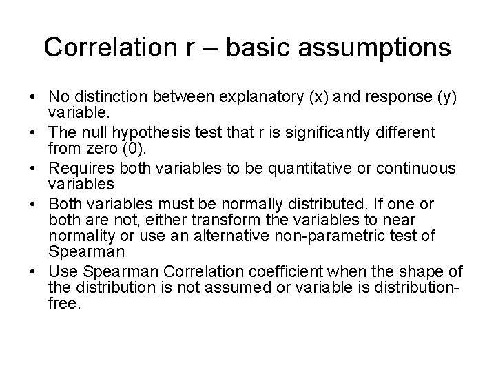
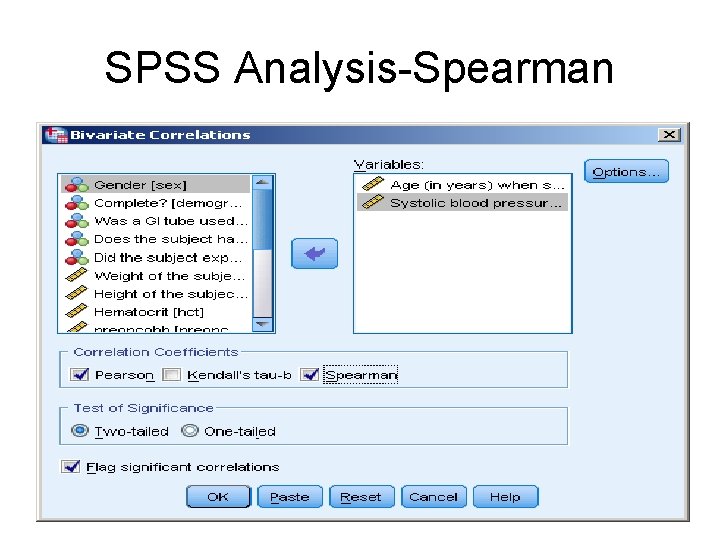
Correlation r – basic assumptions • No distinction between explanatory (x) and response (y) variable. • The null hypothesis test that r is significantly different from zero (0). • Requires both variables to be quantitative or continuous variables • Both variables must be normally distributed. If one or both are not, either transform the variables to near normality or use an alternative non-parametric test of Spearman • Use Spearman Correlation coefficient when the shape of the distribution is not assumed or variable is distributionfree.

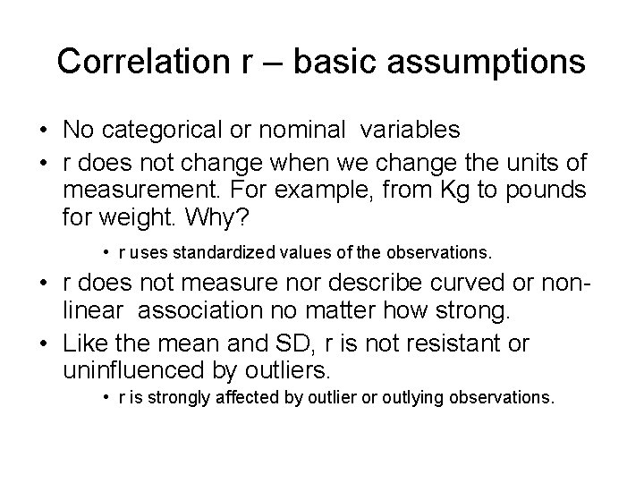
Correlation r – basic assumptions • No categorical or nominal variables • r does not change when we change the units of measurement. For example, from Kg to pounds for weight. Why? • r uses standardized values of the observations. • r does not measure nor describe curved or nonlinear association no matter how strong. • Like the mean and SD, r is not resistant or uninfluenced by outliers. • r is strongly affected by outlier or outlying observations.

Figure 1. Scatter plot of the relationship between SPB and age of children with CP (hypothetical data)

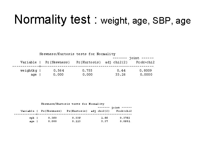
Normality test : weight, age, SBP, age Skewness/Kurtosis tests for Normality ------- joint -----Variable | Pr(Skewness) Pr(Kurtosis) adj chi 2(2) Prob>chi 2 -------+---------------------------weightkg | 0. 564 0. 755 0. 44 0. 8009 age | 0. 000 33. 26 0. 0000 Skewness/Kurtosis tests for Normality ------- joint -----Variable | Pr(Skewness) Pr(Kurtosis) adj chi 2(2) Prob>chi 2 -------+---------------------------spb | 0. 360 0. 339 1. 96 0. 3762 age | 0. 080 0. 113 5. 37 0. 0681

STATA Output – Correlation coefficient (Pearson) • pwcorr spb age, obs sig star(5) • • • | spb age -------+---------spb | 1. 0000 | | 20 | age | 0. 9801* 1. 0000 | 0. 0000 | 20 20 Non-significant correlation does not imply no association

Scatter plot of the relationship between weight and age of children with CP (hypothetical data)

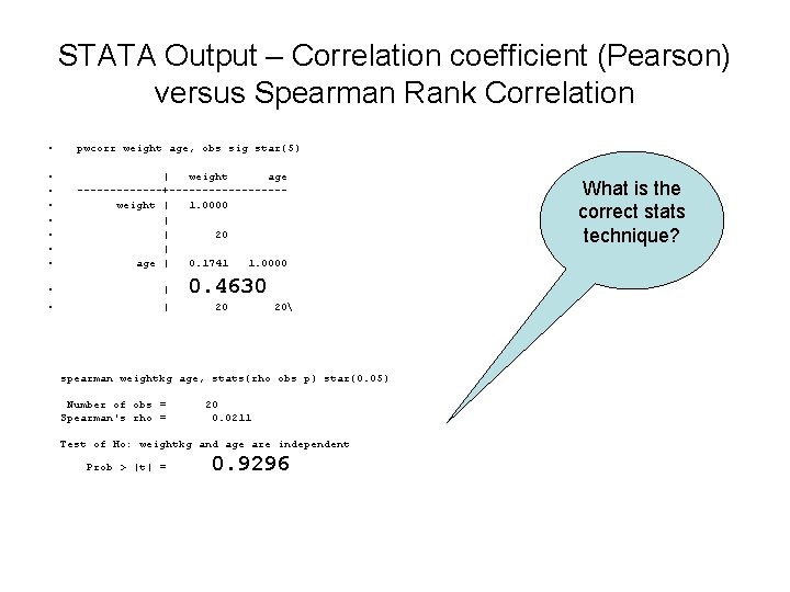
STATA Output – Correlation coefficient (Pearson) versus Spearman Rank Correlation • pwcorr weight age, obs sig star(5) • • | weight age -------+---------weight | 1. 0000 | | 20 | age | 0. 1741 1. 0000 • | 0. 4630 20 20 spearman weightkg age, stats(rho obs p) star(0. 05) Number of obs = Spearman's rho = 20 0. 0211 Test of Ho: weightkg and age are independent Prob > |t| = 0. 9296 What is the correct stats technique?

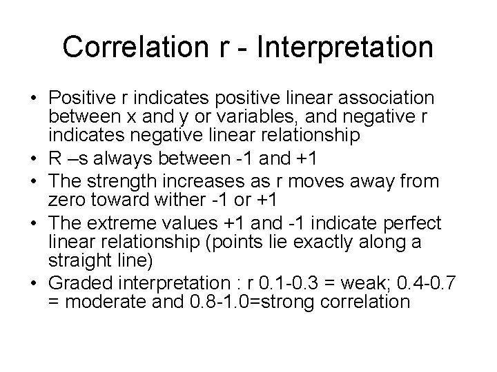
Correlation r - Interpretation • Positive r indicates positive linear association between x and y or variables, and negative r indicates negative linear relationship • R –s always between -1 and +1 • The strength increases as r moves away from zero toward wither -1 or +1 • The extreme values +1 and -1 indicate perfect linear relationship (points lie exactly along a straight line) • Graded interpretation : r 0. 1 -0. 3 = weak; 0. 4 -0. 7 = moderate and 0. 8 -1. 0=strong correlation

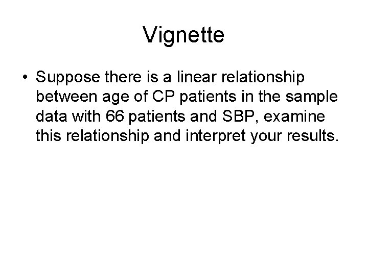
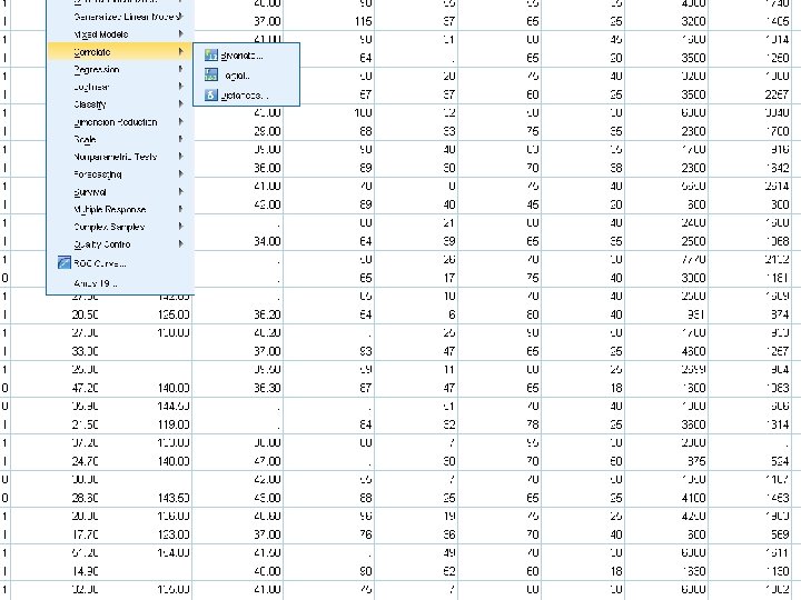
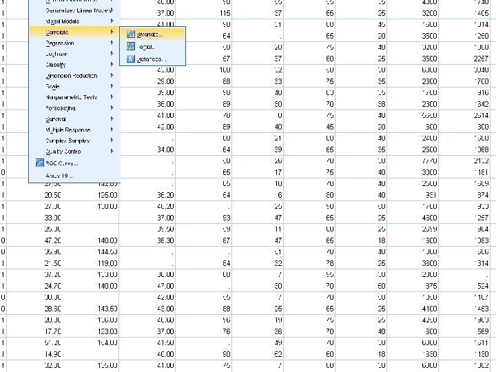
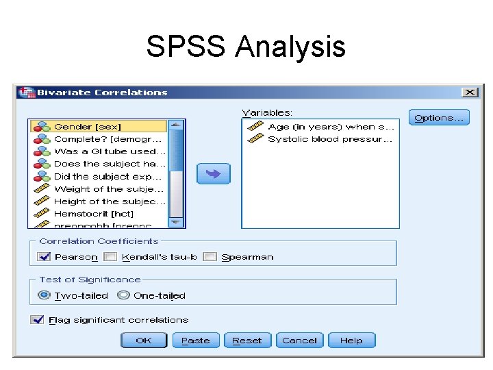
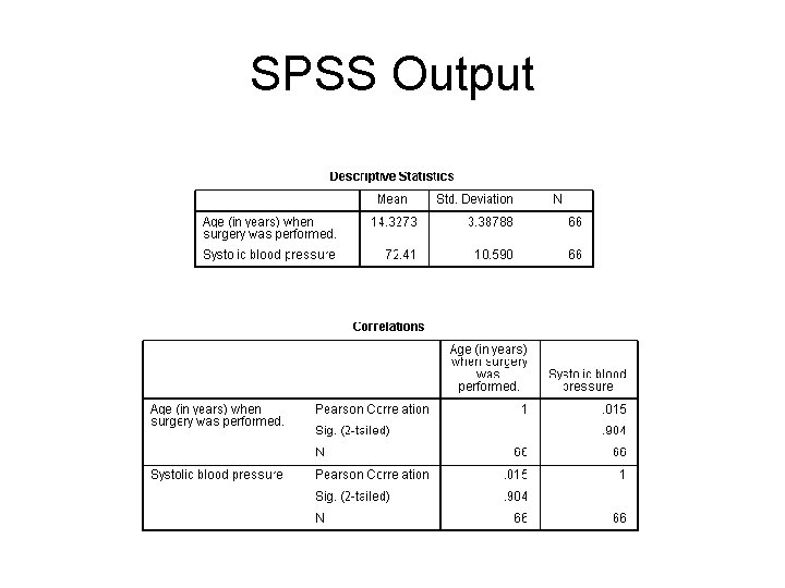
Vignette • Suppose there is a linear relationship between age of CP patients in the sample data with 66 patients and SBP, examine this relationship and interpret your results.

Analysis

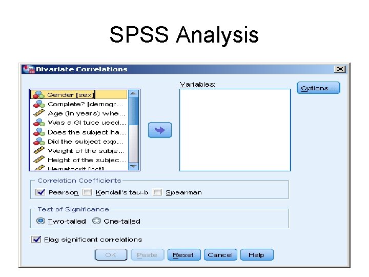
SPSS Analysis

SPSS Analysis

SPSS Output

SPSS Analysis-Spearman

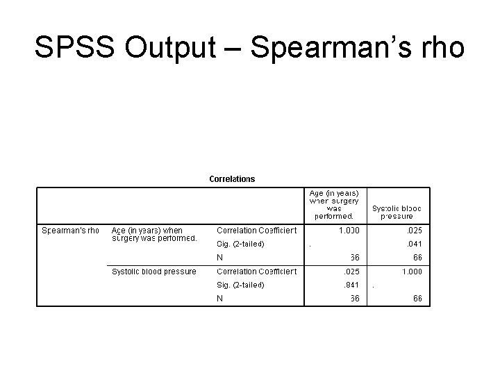
SPSS Output – Spearman’s rho

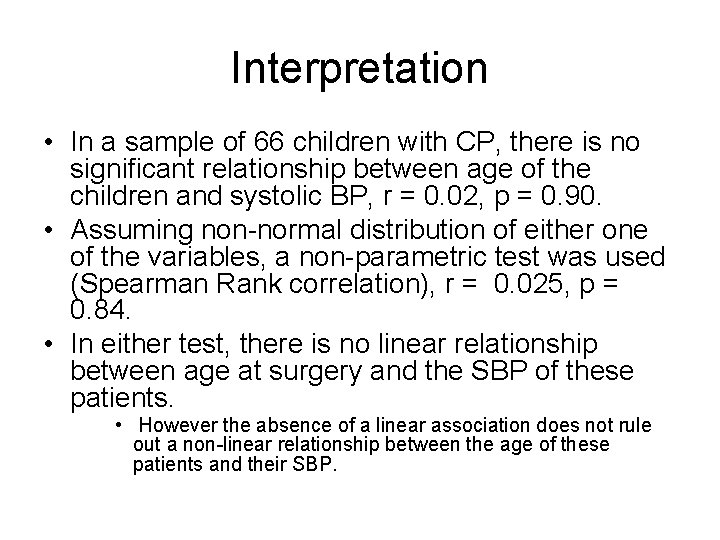
Interpretation • In a sample of 66 children with CP, there is no significant relationship between age of the children and systolic BP, r = 0. 02, p = 0. 90. • Assuming non-normal distribution of either one of the variables, a non-parametric test was used (Spearman Rank correlation), r = 0. 025, p = 0. 84. • In either test, there is no linear relationship between age at surgery and the SBP of these patients. • However the absence of a linear association does not rule out a non-linear relationship between the age of these patients and their SBP.

SLR does is not a measure of association but linear relationship Simple Linear Regression Stats 101 Absence of a significant association in SLR does not imply absence of non-linear association.

Regression Model • Statistical technique for assessing the relationship between dependent and one or more independent variable • The relationship between two variables is characterized by how they vary together. • Given pairs of X and Y variables, regression analysis measures the direction (positive and negative) and the rate of change in Y as X changes (Slope)

Regression Model • Adequate for predicting the value of Y, given X • Inappropriate for assessing the strength of an association between two or more variables • Causal association assumed

Simple regression model • Regression equation and line represent the simple linear equation and describe the shape of the relationship between the variables. • Regression line is the line drawn through scatter plot that test the fitness of the regression model like the coefficient of determination in the model •

Basic Assumptions • Linearity – The relationship between Y and X is linear (straight line relationship) • Residuals are independent and normally distributed • Homosedasticity - The variance of the residuals is equal for all X • There is no measurement error on X (impractical assumption) - < 10% is assumed adequate measurement error.

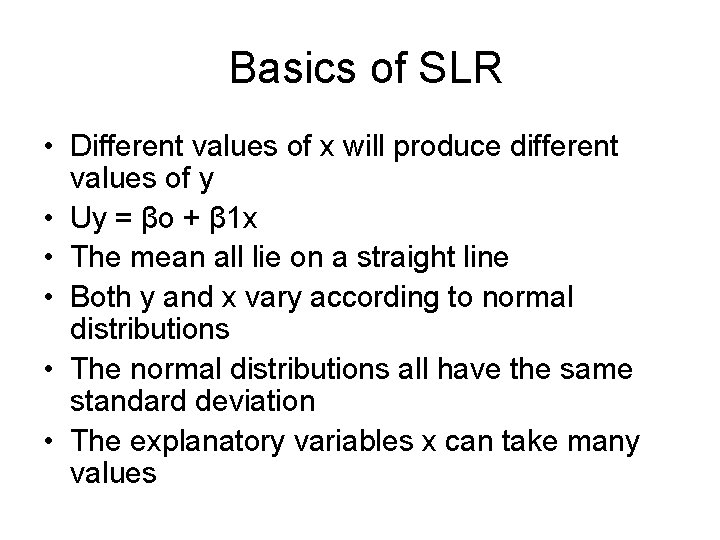
Basics of SLR • Different values of x will produce different values of y • Uy = βo + β 1 x • The mean all lie on a straight line • Both y and x vary according to normal distributions • The normal distributions all have the same standard deviation • The explanatory variables x can take many values

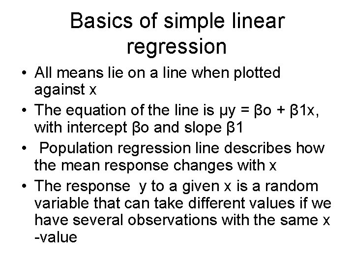
Basics of simple linear regression • All means lie on a line when plotted against x • The equation of the line is μy = βo + β 1 x, with intercept βo and slope β 1 • Population regression line describes how the mean response changes with x • The response y to a given x is a random variable that can take different values if we have several observations with the same x -value

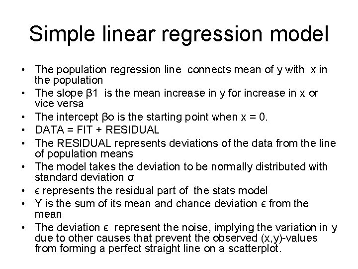
Simple linear regression model • The population regression line connects mean of y with x in the population • The slope β 1 is the mean increase in y for increase in x or vice versa • The intercept βo is the starting point when x = 0. • DATA = FIT + RESIDUAL • The RESIDUAL represents deviations of the data from the line of population means • The model takes the deviation to be normally distributed with standard deviation σ • ϵ represents the residual part of the stats model • Y is the sum of its mean and chance deviation ϵ from the mean • The deviation ϵ represent the noise, implying the variation in y due to other causes that prevent the observed (x, y)-values from forming a perfect straight line on a scatterplot.

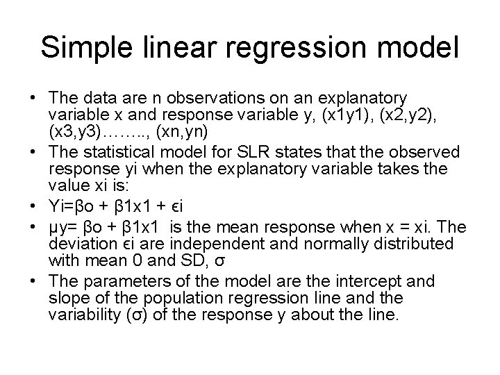
Simple linear regression model • The data are n observations on an explanatory variable x and response variable y, (x 1 y 1), (x 2, y 2), (x 3, y 3)……. . , (xn, yn) • The statistical model for SLR states that the observed response yi when the explanatory variable takes the value xi is: • Yi=βo + β 1 x 1 + ϵi • μy= βo + β 1 x 1 is the mean response when x = xi. The deviation ϵi are independent and normally distributed with mean 0 and SD, σ • The parameters of the model are the intercept and slope of the population regression line and the variability (σ) of the response y about the line.

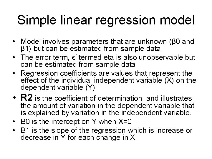
Simple linear regression model • Model involves parameters that are unknown (β 0 and β 1) but can be estimated from sample data • The error term, ϵί termed eta is also unobservable but can be estimated from sample data • Regression coefficients are values that represent the effect of the individual independent variable (X) on the dependent variable (Y) • R 2 is the coefficient of determination and illustrates the amount of variation in the dependent variable that is explained by variation in the independent variable. • Β 0 is the intercept on Y when X=0 • Β 1 is the slope of the regression which is increase or decrease in Y for each change in X.

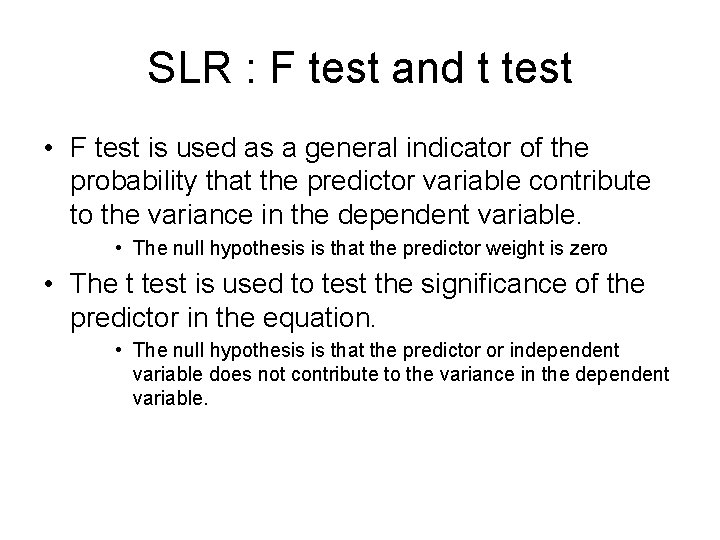
SLR : F test and t test • F test is used as a general indicator of the probability that the predictor variable contribute to the variance in the dependent variable. • The null hypothesis is that the predictor weight is zero • The t test is used to test the significance of the predictor in the equation. • The null hypothesis is that the predictor or independent variable does not contribute to the variance in the dependent variable.

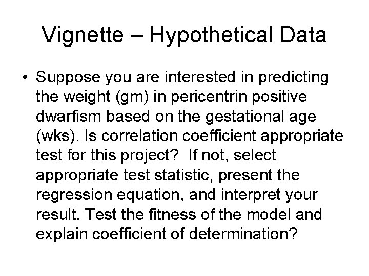
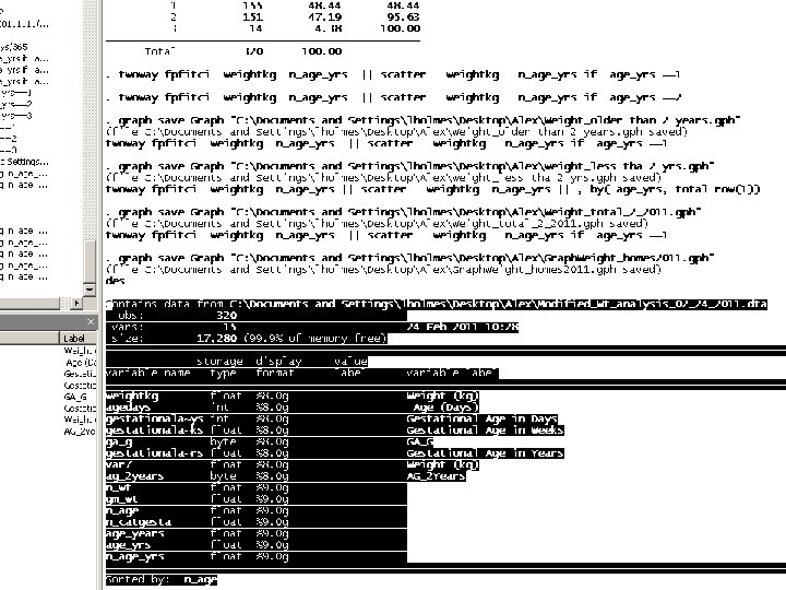
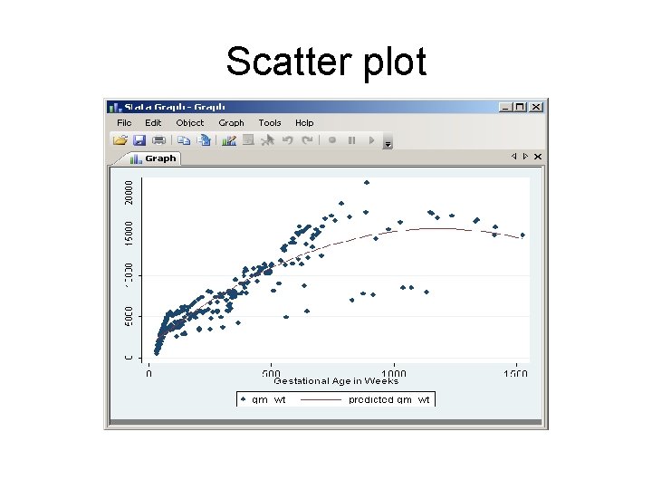
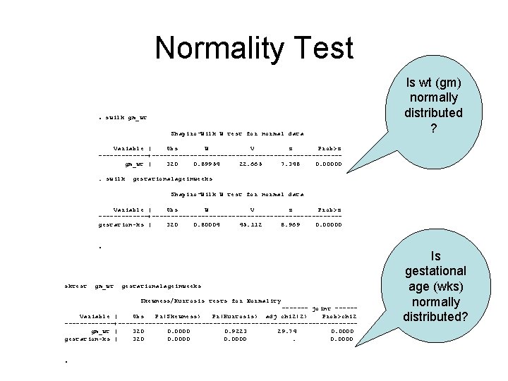
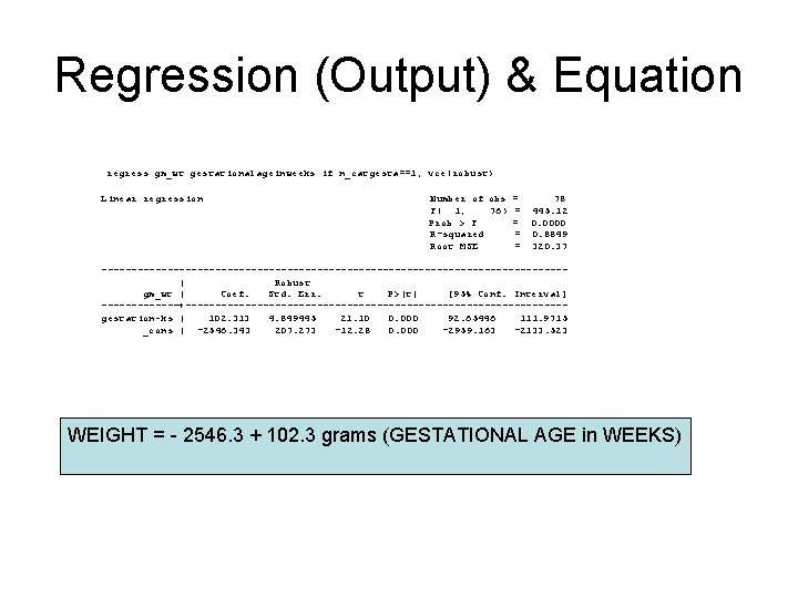
Vignette – Hypothetical Data • Suppose you are interested in predicting the weight (gm) in pericentrin positive dwarfism based on the gestational age (wks). Is correlation coefficient appropriate test for this project? If not, select appropriate test statistic, present the regression equation, and interpret your result. Test the fitness of the model and explain coefficient of determination?

SPSS Analysis

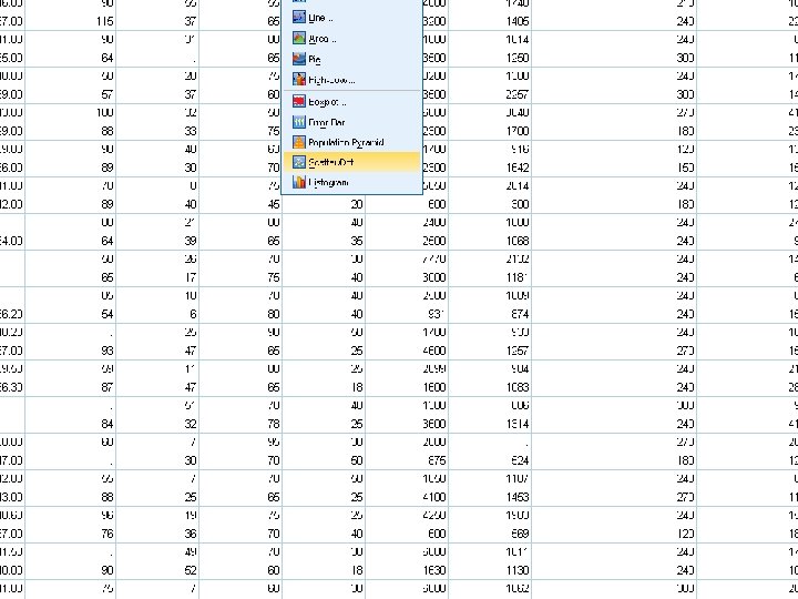
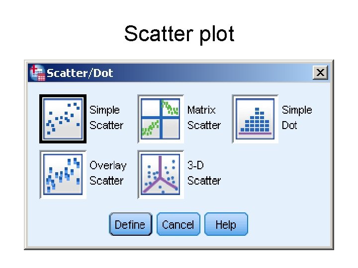
Scatter plot

Normality Test. swilk gm_wt Shapiro-Wilk W test for normal data Is wt (gm) normally distributed ? Variable | Obs W V z Prob>z -------+-------------------------gm_wt | 320 0. 89954 22. 665 7. 348 0. 00000. swilk gestationalageinweeks Shapiro-Wilk W test for normal data Variable | Obs W V z Prob>z -------+-------------------------gestation~ks | 320 0. 80004 45. 112 8. 969 0. 00000 . sktest gm_wt gestationalageinweeks Skewness/Kurtosis tests for Normality ------- joint -----Variable | Obs Pr(Skewness) Pr(Kurtosis) adj chi 2(2) Prob>chi 2 -------+-------------------------------gm_wt | 320 0. 0000 0. 9223 29. 74 0. 0000 gestation~ks | 320 0. 0000 . Is gestational age (wks) normally distributed?

Regression (Output) & Equation regress gm_wt gestationalageinweeks if n_catgesta==1, vce(robust) Linear regression Number of obs = F( 1, 76) = Prob > F = R-squared = Root MSE = 78 445. 12 0. 0000 0. 8849 320. 37 ---------------------------------------| Robust gm_wt | Coef. Std. Err. t P>|t| [95% Conf. Interval] -------+--------------------------------gestation~ks | 102. 313 4. 849445 21. 10 0. 000 92. 65446 111. 9715 _cons | -2546. 343 207. 273 -12. 28 0. 000 -2959. 163 -2133. 523 WEIGHT = - 2546. 3 + 102. 3 grams (GESTATIONAL AGE in WEEKS)

Regression Line, Equation, R square What is R square? Interpret the regression equation

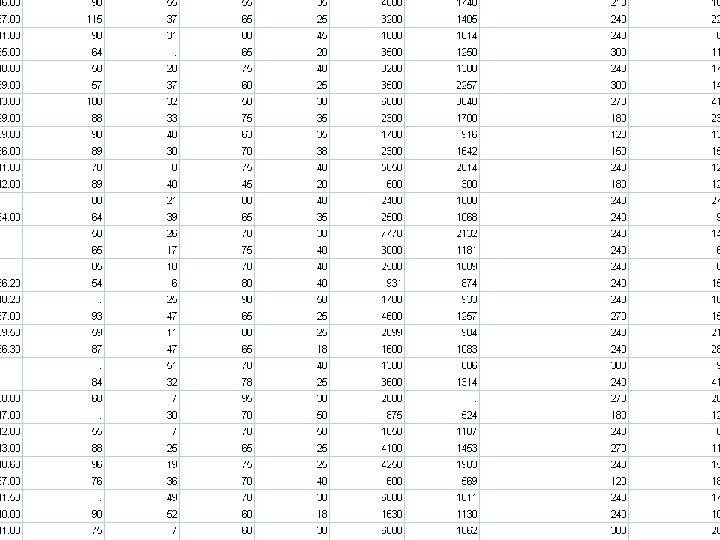
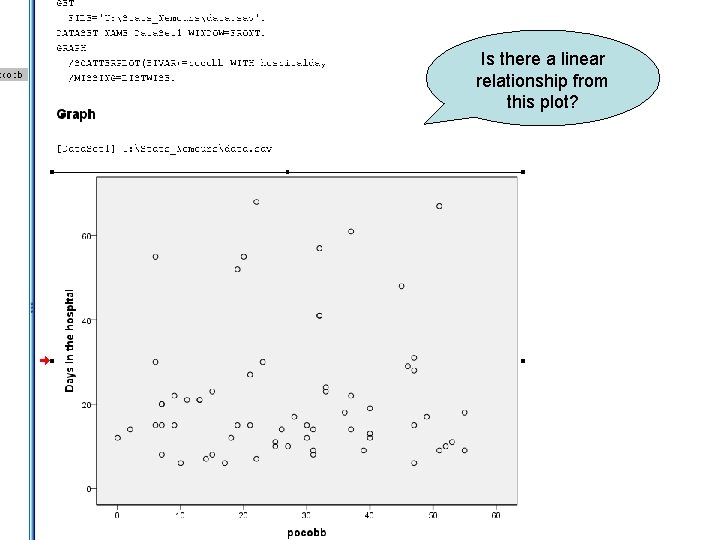
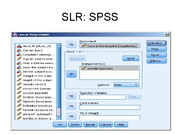
Vignette • In children with CP who underwent spinal fusion for curve deformities correction, can postoperative cobb angle be used in predicting their length of hospitalization? What is the regression equation? Please interpret your result.

Scatter plot

Is there a linear relationship from this plot?

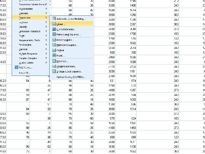
SLR: SPSS

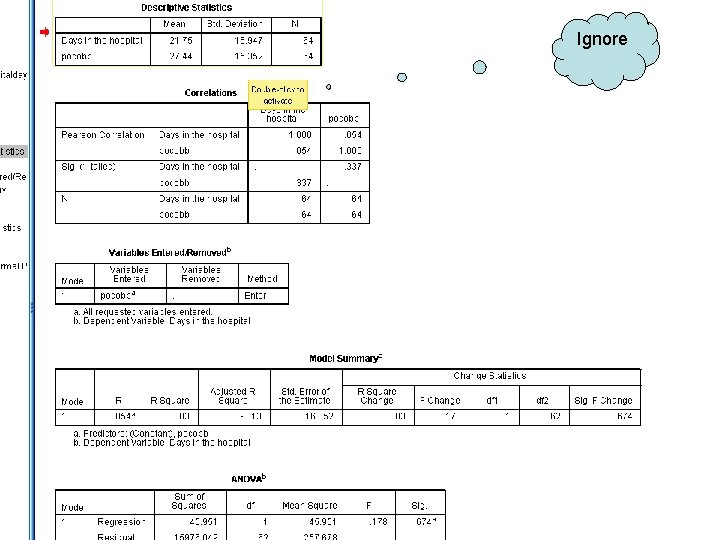
Ignore

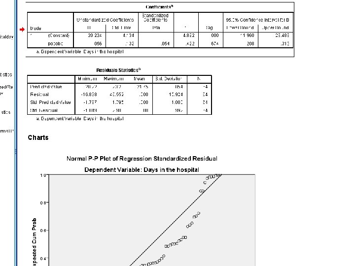
Result Interpretation • The result from SLR states the direction, strength, value, degrees of freedom and significance level. • Note that if ANOVA is not significant, the section of the output labeled sig will be > 0. 05, implying that the regression equation is not significant. • Statement of result: A simple linear regression was computed predicting CP children’s length of hospital stay following spinal fusion based on their postoperative cobb angle. The regression equation was not significant (F( 1, 62)= 0. 18, p = 0. 67, with an R square of 0. 003. • Therefore, postoperative cobb angle cannot be used to predict the length of hospitalization following spinal fusion in CP children with scoliosis.

53