Assignment 4 Problems with parameterization example keeper usage

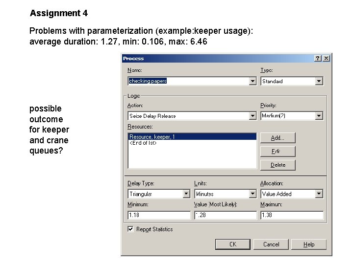
Assignment 4 Problems with parameterization (example: keeper usage): average duration: 1. 27, min: 0. 106, max: 6. 46 possible outcome for keeper and crane queues?

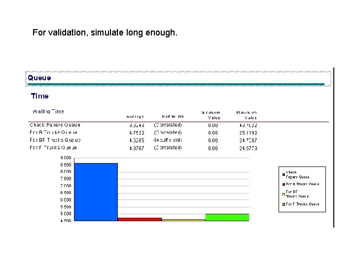
For validation, simulate long enough.

Half widths Half width determination by Arena: statistical analysis of samples. Arena help file: Half Width (Runtime Confidence Intervals—Within a Replication) Some sections contain a column called "Half Width". This statistic is included to help you determine the reliability of the results from your replication. Three results are possible in the "Half Width" category: Insufficient: The formula used to calculate half width requires the samples to be normally distributed. That assumption may be violated if there is a small number (fewer than 320) of samples. If that is the case, Arena will return the message "Insufficient" for that variable’s half width, indicating there is insufficient data to accurately calculate the half width. Running the simulation for a longer period of time should correct this. Correllated: The formula used to calculate half width requires the samples to be independently distributed. Data that is correlated (the value of one observation strongly influences the value of the next observation) results in an invalid confidence interval calculation. If data is determined to be correlated, the message "Correllated" is returned for that variable’s half width. Running the simulation for a longer period of time should correct this. A value: If a value is returned in the Half Width category, this value may be interpreted by saying "in 95% of repeated trials, the sample mean would be reported as within the interval sample mean ± half width".

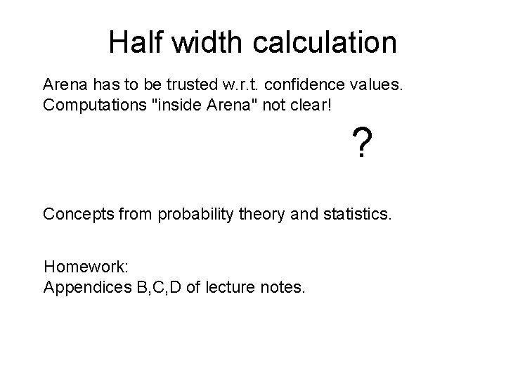
Half width calculation Arena has to be trusted w. r. t. confidence values. Computations "inside Arena" not clear! - determine average and variance s^2 - test for insufficient/correlated - half width = C. s for some constant C. ? Concepts from probability theory and statistics. Homework: Appendices B, C, D of lecture notes.

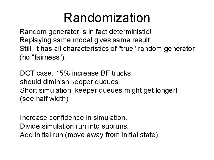
Randomization Random generator is in fact deterministic! Replaying same model gives same result. Still, it has all characteristics of "true" random generator (no "fairness"). DCT case: 15% increase BF trucks should diminish keeper queues. Short simulation: keeper queues might get longer! (see half width) Increase confidence in simulation. Divide simulation run into subruns. Add initial run (move away from initial state).

Replications Make sure that replications/subruns are independent (e. g. no queue length dependencies). When done right, division into subruns allows to compute confidence intervals. Example computation: page 30 of lecture notes. n = 30 subruns, each with sample of measure x (occupation rate).

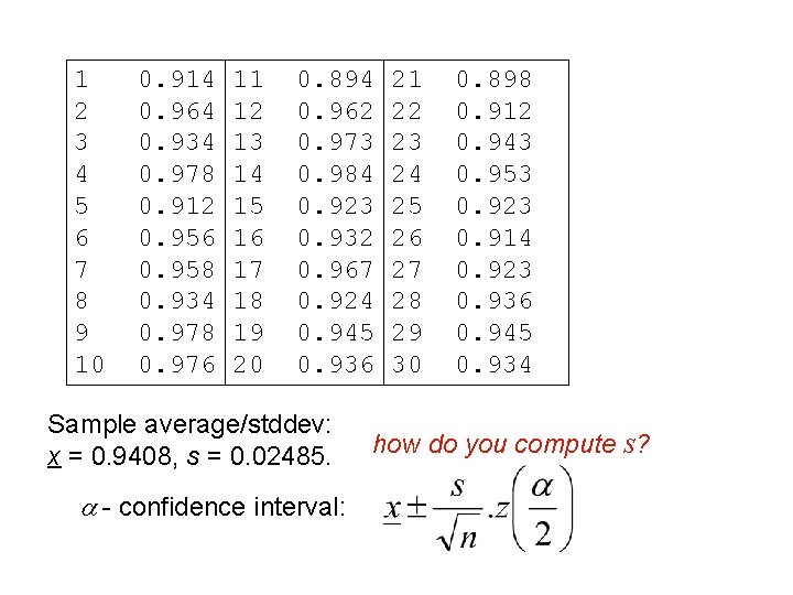
1 2 3 4 5 6 7 8 9 10 0. 914 0. 964 0. 934 0. 978 0. 912 0. 956 0. 958 0. 934 0. 978 0. 976 11 12 13 14 15 16 17 18 19 20 0. 894 0. 962 0. 973 0. 984 0. 923 0. 932 0. 967 0. 924 0. 945 0. 936 Sample average/stddev: x = 0. 9408, s = 0. 02485. a - confidence interval: 21 22 23 24 25 26 27 28 29 30 0. 898 0. 912 0. 943 0. 953 0. 923 0. 914 0. 923 0. 936 0. 945 0. 934 how do you compute s?

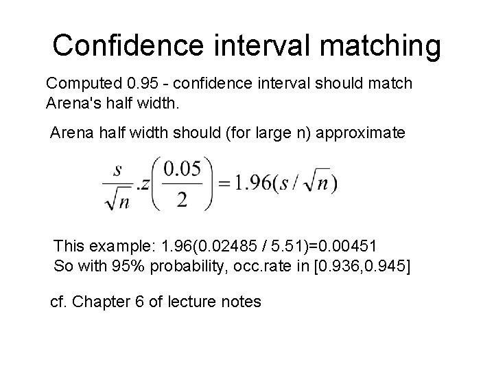
Confidence interval matching Computed 0. 95 - confidence interval should match Arena's half width. Arena half width should (for large n) approximate This example: 1. 96(0. 02485 / 5. 51)=0. 00451 So with 95% probability, occ. rate in [0. 936, 0. 945] cf. Chapter 6 of lecture notes

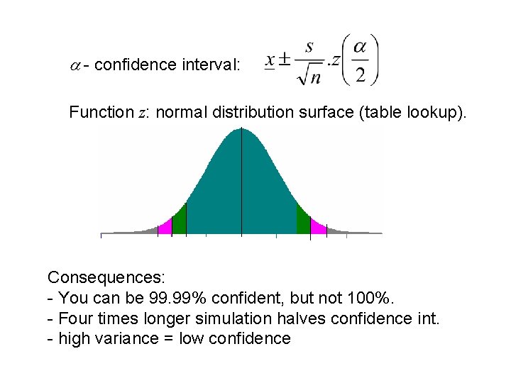
a - confidence interval: Function z: normal distribution surface (table lookup). Consequences: - You can be 99. 99% confident, but not 100%. - Four times longer simulation halves confidence int. - high variance = low confidence

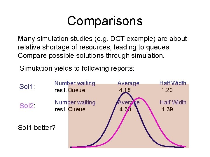
Comparisons Many simulation studies (e. g. DCT example) are about relative shortage of resources, leading to queues. Compare possible solutions through simulation. Simulation yields to following reports: Sol 1: Number waiting res 1. Queue Average 4. 18 Half Width 1. 20 Sol 2: Number waiting res 1. Queue Average 4. 58 Half Width 1. 39 Sol 1 better?

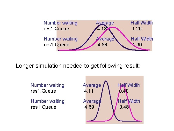
Number waiting res 1. Queue Average 4. 18 Half Width 1. 20 Number waiting res 1. Queue Average 4. 58 Half Width 1. 39 Longer simulation needed to get following result: Number waiting res 1. Queue Average 4. 11 Half Width 0. 40 Number waiting res 1. Queue Average 4. 69 Half Width 0. 48

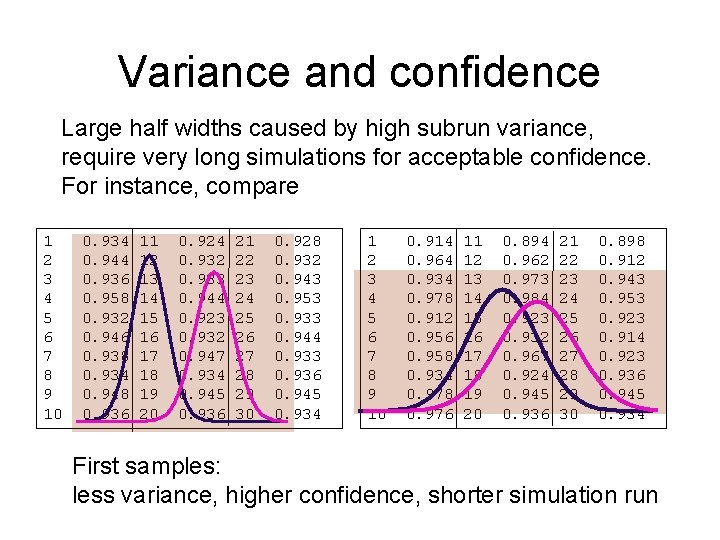
Variance and confidence Large half widths caused by high subrun variance, require very long simulations for acceptable confidence. For instance, compare 1 2 3 4 5 6 7 8 9 10 0. 934 0. 944 0. 936 0. 958 0. 932 0. 946 0. 938 0. 934 0. 948 0. 936 11 12 13 14 15 16 17 18 19 20 0. 924 0. 932 0. 933 0. 944 0. 923 0. 932 0. 947 0. 934 0. 945 0. 936 21 22 23 24 25 26 27 28 29 30 0. 928 0. 932 0. 943 0. 953 0. 933 0. 944 0. 933 0. 936 0. 945 0. 934 1 2 3 4 5 6 7 8 9 10 0. 914 0. 964 0. 934 0. 978 0. 912 0. 956 0. 958 0. 934 0. 978 0. 976 11 12 13 14 15 16 17 18 19 20 0. 894 0. 962 0. 973 0. 984 0. 923 0. 932 0. 967 0. 924 0. 945 0. 936 21 22 23 24 25 26 27 28 29 30 0. 898 0. 912 0. 943 0. 953 0. 923 0. 914 0. 923 0. 936 0. 945 0. 934 First samples: less variance, higher confidence, shorter simulation run

Variance reduction 1 Large half widths caused by high subrun variance, require very long simulations for acceptable confidence. Various techniques to reduce subrun variance, e. g. antithetic random numbers (see lecture notes) Subrun result depends on sequence of random numbers Next subrun: use antithetic sequence: Frequent arrivals, long processing times in a subrun compensated by infrequent arrivals and short times in next subrun.

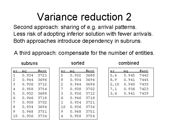
Variance reduction 2 Second approach: sharing of e. g. arrival patterns. Less risk of adopting inferior solution with fewer arrivals. Both approaches introduce dependency in subruns. A third approach: compensate for the number of entities. sorted subruns sr 1 2 3 4 5 6 7 8 9 10 mq 0. 934 0. 944 0. 936 0. 958 0. 932 0. 946 0. 938 0. 934 0. 948 0. 936 #ent 3721 3696 3712 3754 3688 3718 3702 3694 3751 3734 sr 5 8 2 7 3 6 1 10 9 4 mq 0. 932 0. 934 0. 944 0. 938 0. 936 0. 946 0. 934 0. 936 0. 948 0. 958 combined #ent 3688 3694 3696 3702 3718 3721 3734 3751 3754 sr 5, 4 8, 9 2, 10 7, 1 3, 6 mq 0. 945 0. 941 0. 940 0. 936 0. 941 #ent 7442 7445 7430 7423 7439

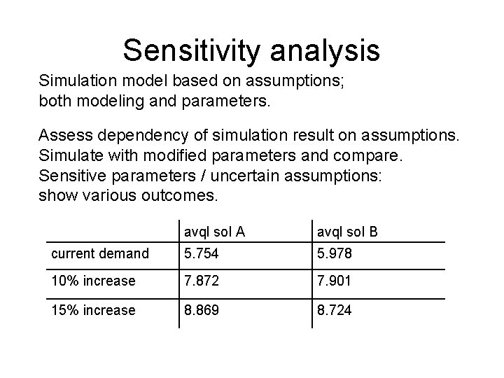
Sensitivity analysis Simulation model based on assumptions; both modeling and parameters. Assess dependency of simulation result on assumptions. Simulate with modified parameters and compare. Sensitive parameters / uncertain assumptions: show various outcomes. avql sol A avql sol B current demand 5. 754 5. 978 10% increase 7. 872 7. 901 15% increase 8. 869 8. 724