Assessment On the VLE Module Assessment link ii

Assessment On the VLE Module Assessment link (ii) A report of the summer term Experimental Design Practical including an Appendix with R script. • logical folder structure • script, any accessory functions and the data itself. • script should be well-commented, well-organised and follow good practice in the use of spacing, indentation, and variable naming. • include all the code required to reproduce data import and formatting as well as the summary information, analyses, and figures in your report. • Examples of well-formatted scripts are given at the end of most workshops. 1

Laboratory & Professional skills for Bioscientists Term 2: Data Analysis in R Two sample tests: two-sample t-test, two-sample Wilcoxon Practical: one and two sample tests examples, different data formats ggplot. 2

Summary • Tests for one-, two-, and paired-samples (ttests and non-parametric equivalents) • Today – two-sample t-test for independent samples – Wilcoxon for one- and two-samples when t-test assumptions are not met • Choosing appropriate tests: type of question, type of data • Second of two lectures; single workshop 3

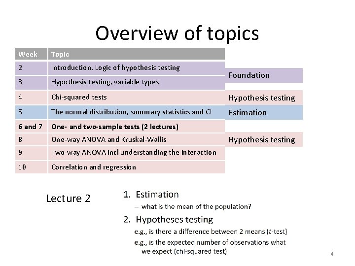
Overview of topics Week Topic 2 Introduction. Logic of hypothesis testing 3 Hypothesis testing, variable types 4 Chi-squared tests Hypothesis testing 5 The normal distribution, summary statistics and CI Estimation 6 and 7 One- and two-sample tests (2 lectures) 8 One-way ANOVA and Kruskal-Wallis 9 Two-way ANOVA incl understanding the interaction 10 Correlation and regression Foundation Hypothesis testing Lecture 2 4

le s u e r u ct o i v re p n i o Learning objectives Als By actively following the lecture and practical and carrying out the independent study the successful student will be able to: • Explain dependent and independent samples (MLO 2) • Select, appropriately, t-tests and their nonparametric equivalents (MLO 2) • Apply, interpret and evaluate the legitimacy of the tests in R (MLO 3 and 4) • Summarise and illustrate with appropriate figures test results scientifically (MLO 3 and 4) 5

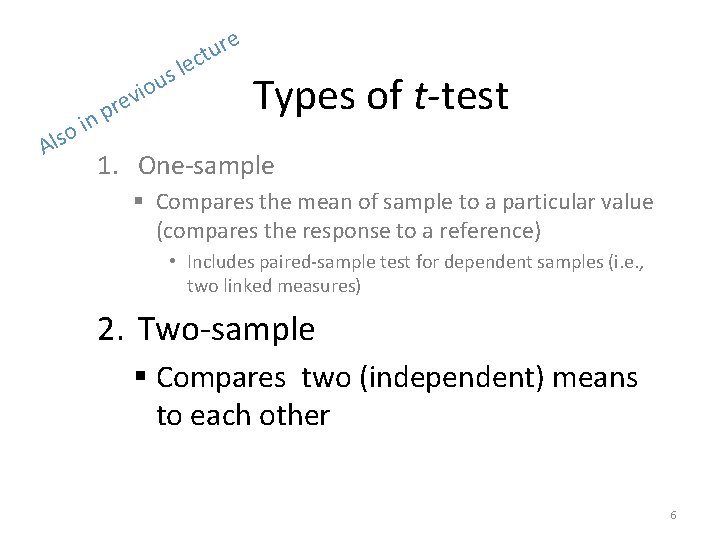
e r u ct le s u o Als o i v re p in Types of t-test 1. One-sample § Compares the mean of sample to a particular value (compares the response to a reference) • Includes paired-sample test for dependent samples (i. e. , two linked measures) 2. Two-sample § Compares two (independent) means to each other 6

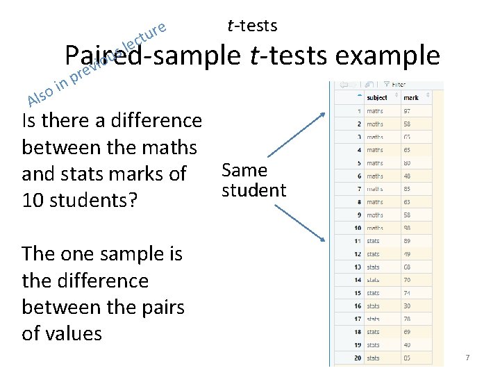
e r u ct le s u t-tests Paired-sample t-tests example o i v re p n i o Als Is there a difference between the maths Same and stats marks of student 10 students? The one sample is the difference between the pairs of values 7

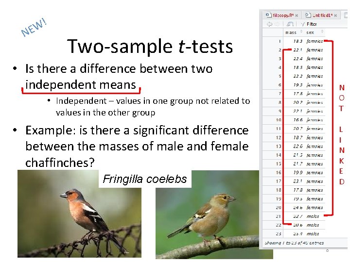
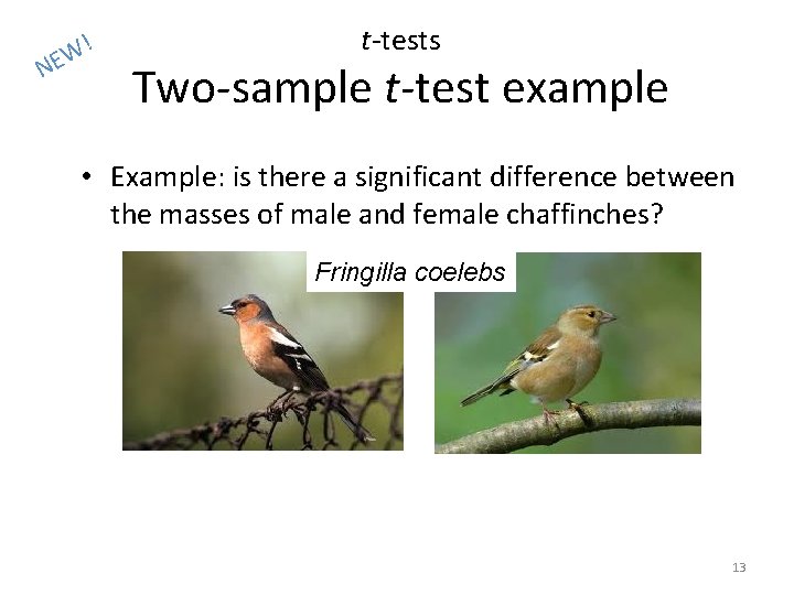
! W E N Two-sample t-tests • Is there a difference between two independent means N O T • Independent – values in one group not related to values in the other group • Example: is there a significant difference between the masses of male and female chaffinches? L I N K E D Fringilla coelebs 8

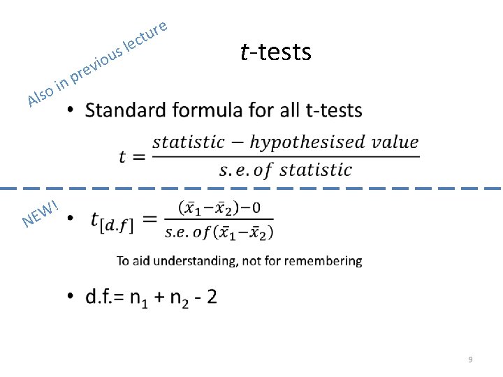
o s l A r p in o i v e le s u e r u ct t-tests • ! W NE 9

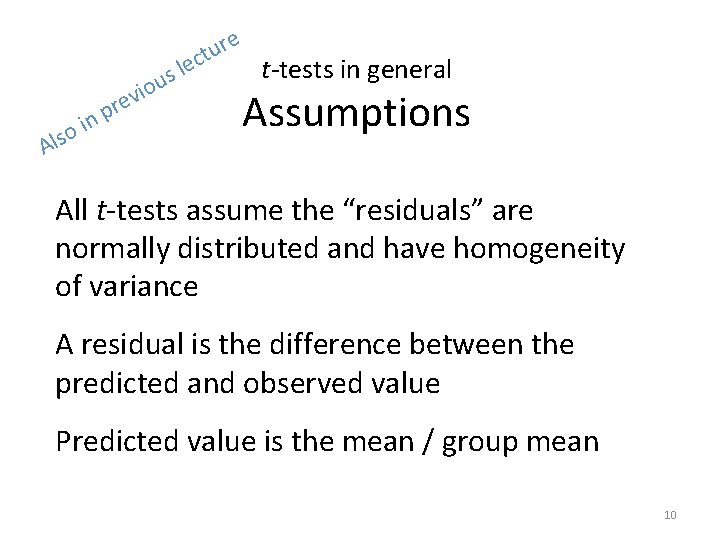
le s u e r u ct o Als o i v re p in t-tests in general Assumptions All t-tests assume the “residuals” are normally distributed and have homogeneity of variance A residual is the difference between the predicted and observed value Predicted value is the mean / group mean 10

e o s l A r p in us o i ev r u t-tests in general: assumptions t c e l Checking Assumptions - Common sense – response should be continuous – No/few repeats - Plot the residuals - Using a test in R 11

re t-tests in general: assumptions u t lec s udata o When are not normally distributed i v e r Als p n i o • Transform (not really covered) § E. g. Log to remove skew, arcsin squareroot on proportions • Use a non-parametric test (covered) § Fewer assumptions § Generally less powerful 12

N ! W E t-tests Two-sample t-test example • Example: is there a significant difference between the masses of male and female chaffinches? Fringilla coelebs 13

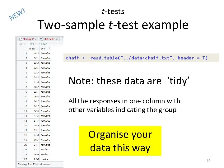
N ! W E t-tests Two-sample t-test example chaff <- read. table(". . /data/chaff. txt", header = T) Note: these data are ‘tidy’ All the responses in one column with other variables indicating the group Organise your data this way 14

u ct e l s s n e t x E o n io o i v re p f Tidy data • Each variable should be in one column. • Each different observation of that variable should be in a different row. • There should be one table for each "kind" of variable. • If you have multiple tables, they should include a column in the table that allows them to be linked. Independent study: Wickham, H (2013). Tidy Data. Journal of Statistical Software. https: //www. jstatsoft. org/article/view/v 059 i 10 15

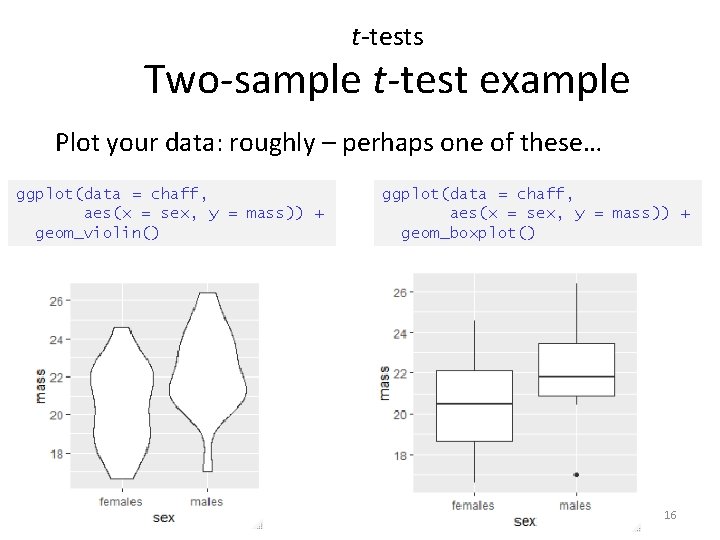
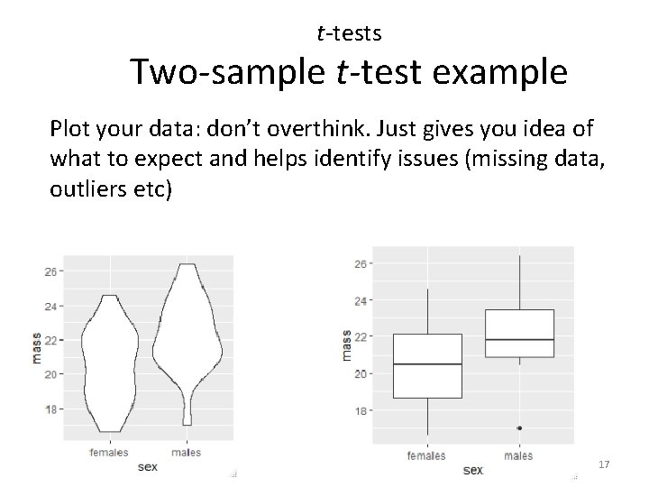
t-tests Two-sample t-test example Plot your data: roughly – perhaps one of these… ggplot(data = chaff, aes(x = sex, y = mass)) + geom_violin() ggplot(data = chaff, aes(x = sex, y = mass)) + geom_boxplot() 16

t-tests Two-sample t-test example Plot your data: don’t overthink. Just gives you idea of what to expect and helps identify issues (missing data, outliers etc) 17

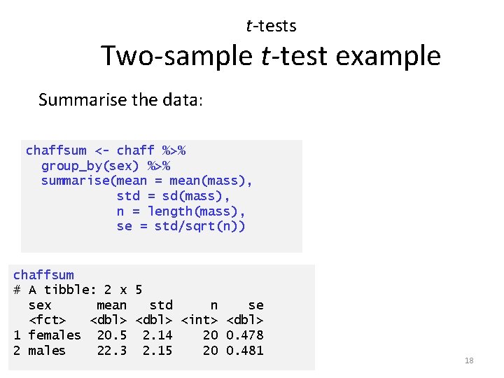
t-tests Two-sample t-test example Summarise the data: chaffsum <- chaff %>% group_by(sex) %>% summarise(mean = mean(mass), std = sd(mass), n = length(mass), se = std/sqrt(n)) chaffsum # A tibble: 2 x 5 sex mean std n se <fct> <dbl> <int> <dbl> 1 females 20. 5 2. 14 20 0. 478 2 males 22. 3 2. 15 20 0. 481 18

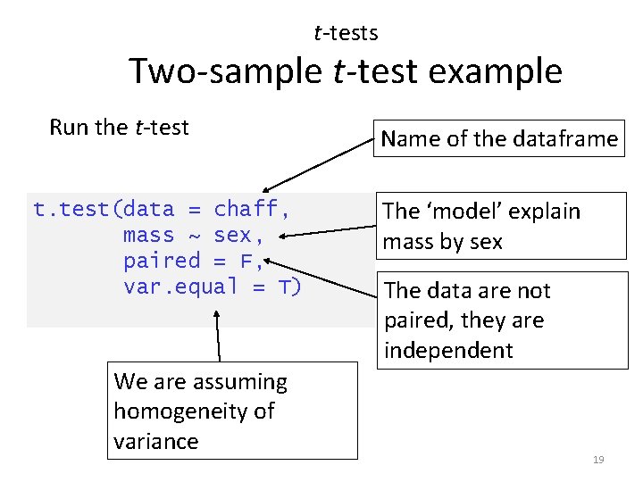
t-tests Two-sample t-test example Run the t-test t. test(data = chaff, mass ~ sex, paired = F, var. equal = T) We are assuming homogeneity of variance Name of the dataframe The ‘model’ explain mass by sex The data are not paired, they are independent 19

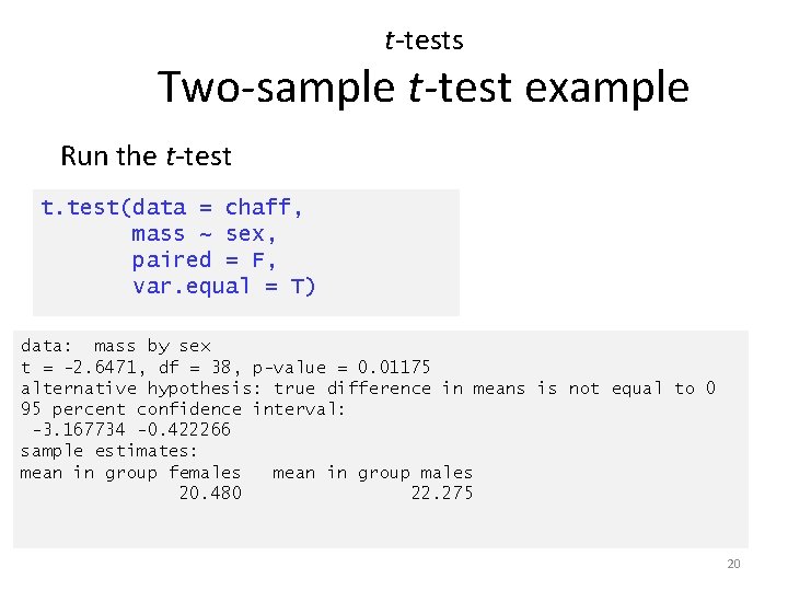
t-tests Two-sample t-test example Run the t-test t. test(data = chaff, mass ~ sex, paired = F, var. equal = T) data: mass by sex t = -2. 6471, df = 38, p-value = 0. 01175 alternative hypothesis: true difference in means is not equal to 0 95 percent confidence interval: -3. 167734 -0. 422266 sample estimates: mean in group females mean in group males 20. 480 22. 275 20

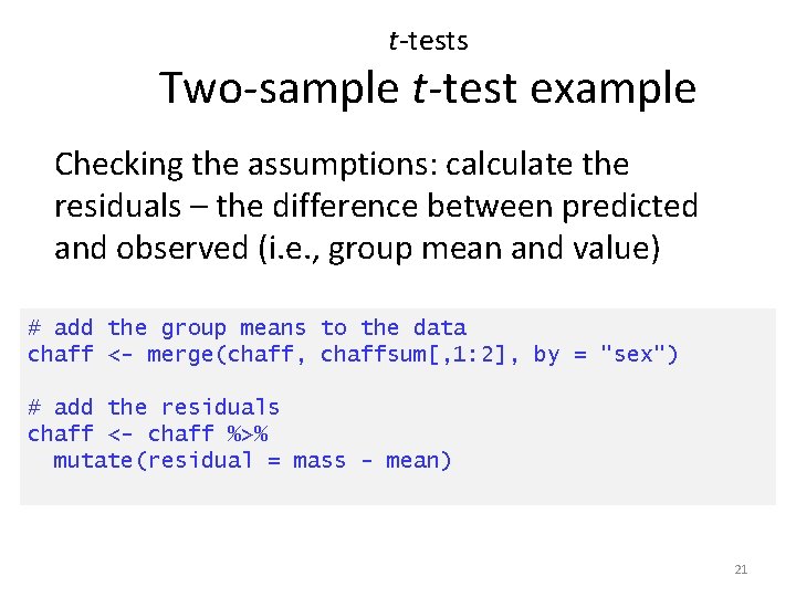
t-tests Two-sample t-test example Checking the assumptions: calculate the residuals – the difference between predicted and observed (i. e. , group mean and value) # add the group means to the data chaff <- merge(chaff, chaffsum[, 1: 2], by = "sex") # add the residuals chaff <- chaff %>% mutate(residual = mass - mean) 21

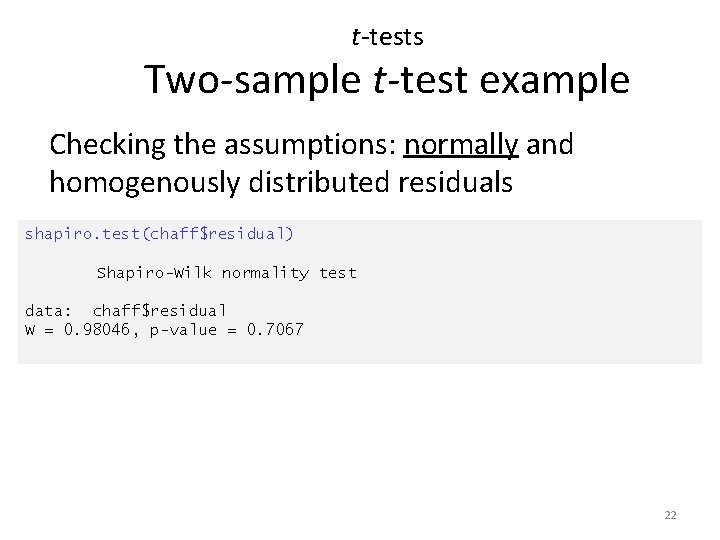
t-tests Two-sample t-test example Checking the assumptions: normally and homogenously distributed residuals shapiro. test(chaff$residual) Shapiro-Wilk normality test data: chaff$residual W = 0. 98046, p-value = 0. 7067 22

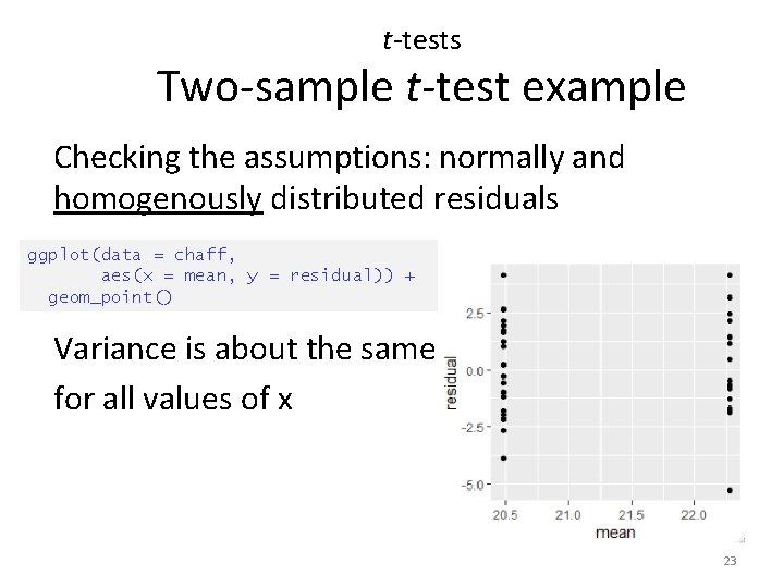
t-tests Two-sample t-test example Checking the assumptions: normally and homogenously distributed residuals ggplot(data = chaff, aes(x = mean, y = residual)) + geom_point() Variance is about the same for all values of x 23

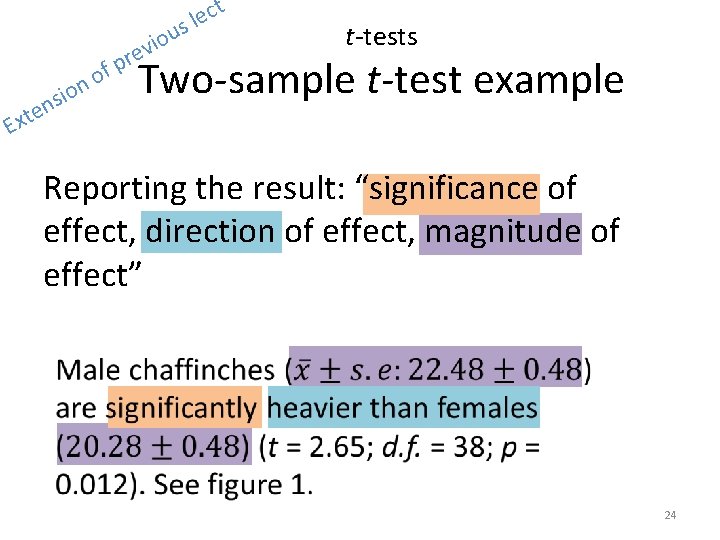
u ct e l s e t x E o nsi o i v re p f t-tests Two-sample t-test example Reporting the result: “significance of effect, direction of effect, magnitude of effect” 24

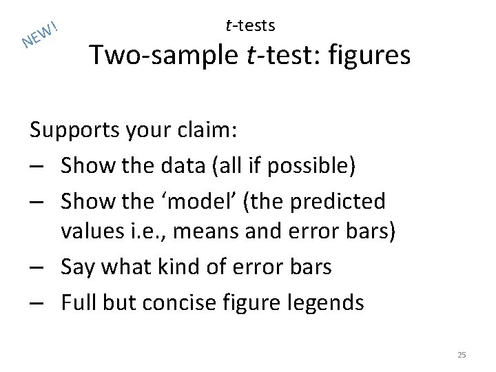
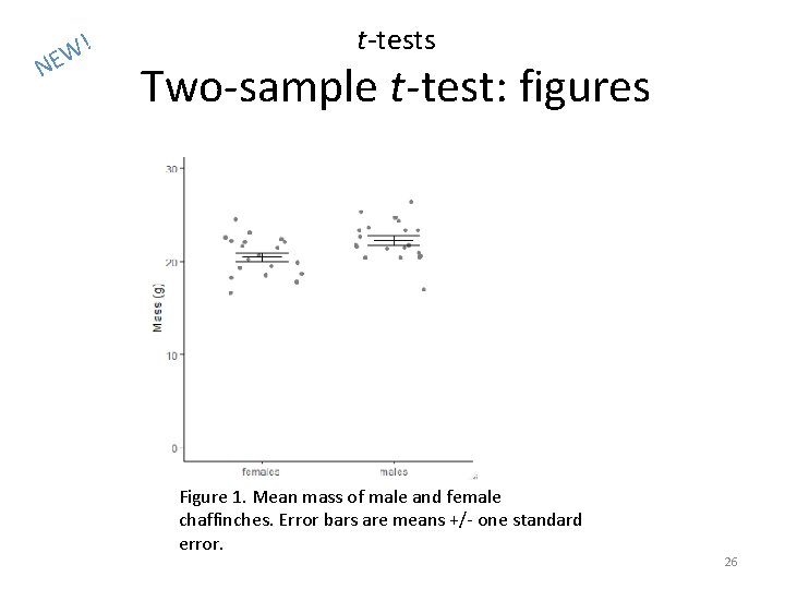
! W E N t-tests Two-sample t-test: figures Supports your claim: – Show the data (all if possible) – Show the ‘model’ (the predicted values i. e. , means and error bars) – Say what kind of error bars – Full but concise figure legends 25

N ! W E t-tests Two-sample t-test: figures Figure 1. Mean mass of male and female chaffinches. Error bars are means +/- one standard error. 26

! W E N Figure 1. Graph to show mass of male and female chaffinches. Error bars are means +/- one standard error. 27

When the t-test assumptions are not met: non- parametric tests • Non-parametric tests make fewer assumptions • Based on the ranks rather than the actual data • Null hypotheses are about the mean rank (not the mean) 28

Non-parametric tests t-test equivalents i, . e. , the type of question is the same but the response variable is not normally distributed • one – sample t-test and paired-sample t-test: the one-sample Wilcoxon • Two-sample t-test: two-sample Wilcoxon aka Mann-Whitney 29

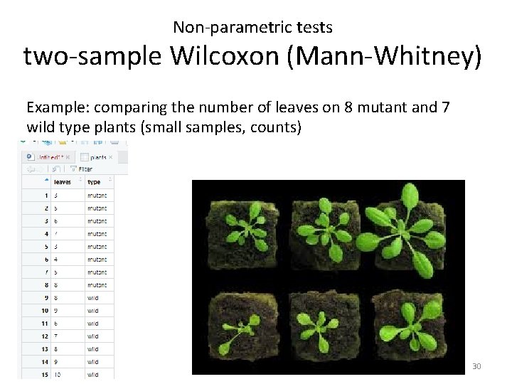
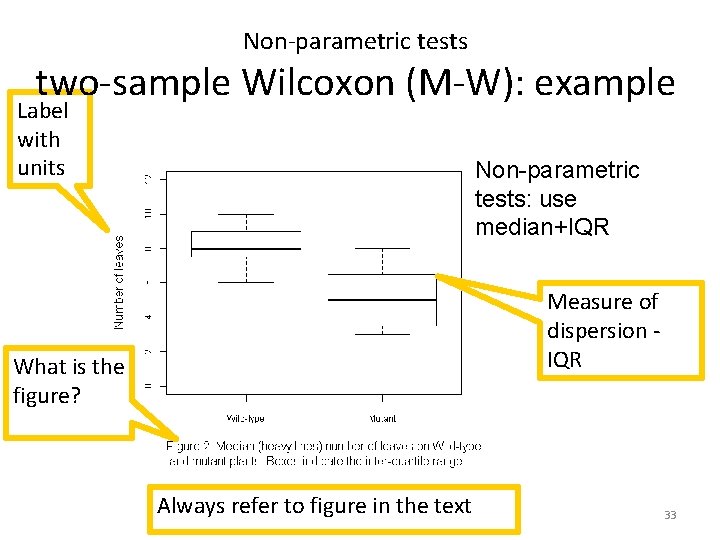
Non-parametric tests two-sample Wilcoxon (Mann-Whitney) Example: comparing the number of leaves on 8 mutant and 7 wild type plants (small samples, counts) 30

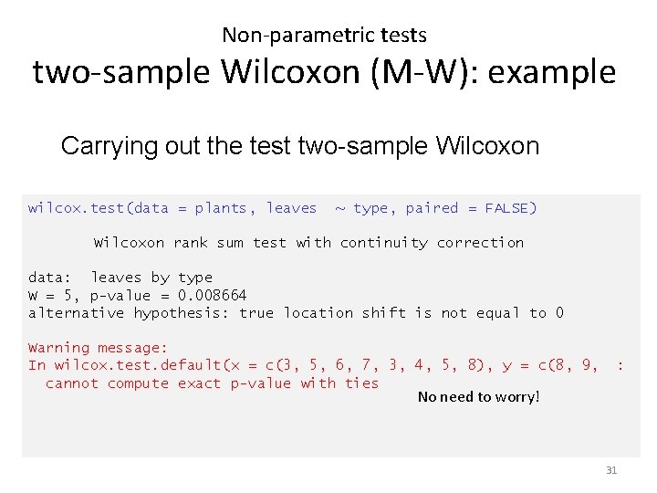
Non-parametric tests two-sample Wilcoxon (M-W): example Carrying out the test two-sample Wilcoxon wilcox. test(data = plants, leaves ~ type, paired = FALSE) Wilcoxon rank sum test with continuity correction data: leaves by type W = 5, p-value = 0. 008664 alternative hypothesis: true location shift is not equal to 0 Warning message: In wilcox. test. default(x = c(3, 5, 6, 7, 3, 4, 5, 8), y = c(8, 9, cannot compute exact p-value with ties : No need to worry! 31

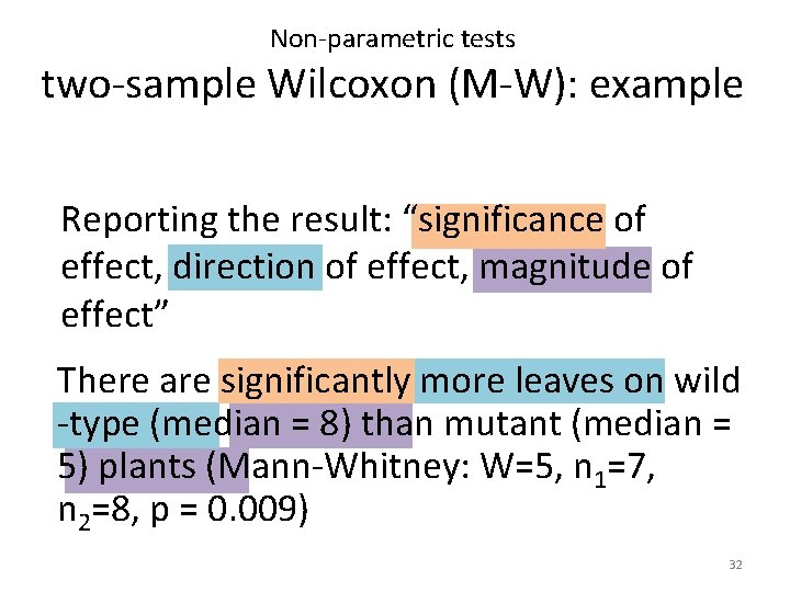
Non-parametric tests two-sample Wilcoxon (M-W): example Reporting the result: “significance of effect, direction of effect, magnitude of effect” There are significantly more leaves on wild -type (median = 8) than mutant (median = 5) plants (Mann-Whitney: W=5, n 1=7, n 2=8, p = 0. 009) 32

Non-parametric tests two-sample Wilcoxon (M-W): example Label with units Non-parametric tests: use median+IQR Measure of dispersion IQR What is the figure? Always refer to figure in the text 33

Learning objectives for the week By attending the lectures and practical the successful student will be able to • Explain dependent and independent samples (MLO 2) • Select, appropriately, t-tests and their nonparametric equivalents (MLO 2) • Apply, interpret and evaluate the legitimacy of the tests in R (MLO 3 and 4) • Summarise and illustrate with appropriate R figures test results scientifically (MLO 3 and 4) 34