Assessing the GIA Contribution to SNARF Mark Tamisiea

Assessing the GIA Contribution to SNARF �Mark Tamisiea and Jim Davis Harvard-Smithsonian Center for Astrophysics
 of GIA field in SNARF 1. 0 • Inclusion of")
Outline • Review (background) of GIA field in SNARF 1. 0 • Inclusion of GRACE data • Radial (and geoid) only solutions • Discussion – How the product will be used – How to assign/use/interpret rotational and translational terms

GIA Predictions: Requirements • A model for the Earth’s viscoelastic structure • A history of the time-dependent ice load • Theory and code to convolve the time-dependent load with the viscoelastic Green’s functions, while simultaneously solving for effects due to the redistribution of the surface load (ice water)

GIA Predictions: Practical Issues • Uncertainties in viscosity structure and ice history • Ice & Earth models are generally not independent (inversions nonunique) • Generally, Earth models used to generate GIA predictions are spherically symmetric, but lateral variations are important
 • Combine data")
New Approach • Treat model predictions as statistical quantities (Bayesian approach) • Combine data and models using assimilation techniques (Kalman filter) • How do we get model “uncertainties”? • Calculate field mean, covariance over suite of reasonable Earth, ice models

Model Covariances • Example: covariance of east component of deformation at point 1 with radial component of deformation at point 2: • Covariance matrix has “physics” of GIA

Prior Correlatio�n wrt ALGO

Definitions and Assumptions • Given a geodetic solution with site velocities VGPS at locations (l, f), we can describe the solution using • The velocity rotation and translation parameters are unknown and must be estimated as part of the SNARF definition

GPS Data Assimilation • We simultaneously estimate six rotation and translation parameters, and GIA velocities at n grid locations and at m GPS sites • At right, the parameter vector (u = east velocity, v = north, w = radial) • The observations consist of (u, v, w) for GPS sites • The GIA values at the grid locations are adjusted through the covariances calculated from the suite of model predictions
![Assimilation (SNARF 1. 0) • Ice model: Ice-1 [Peltier & Andrews, 1976] • Earth](http://slidetodoc.com/presentation_image/fbe1fa5d6424dc3bb3f93e22dbc51a4e/image-10.jpg "Assimilation (SNARF 1. 0) • Ice model: Ice-1 [Peltier & Andrews, 1976] • Earth")
Assimilation (SNARF 1. 0) • Ice model: Ice-1 [Peltier & Andrews, 1976] • Earth models: Spherically symmetric threelayer, range of elastic lithospheric thicknesses, upper and lower mantle viscosities (see Milne et al. , 2001) • Elastic parameters: PREM • GPS data set: Velocities from “good” GPS sites, NAREF solution from Mike Craymer • Placed in approximate NA frame by Tom Herring (unnecessary step but simpler)
: 1. 22 mm/yr WRMS (rad):")
SNARF 1. 0 GIA Field Prefit statistics: WRMS (hor): 1. 22 mm/yr WRMS (rad): 3. 81 mm/yr WRMS (all): 1. 74 mm/yr Postfit statistics: WRMS (hor): 0. 71 mm/yr WRMS (rad): 1. 30 mm/yr WRMS (all): 0. 80 mm/yr
![Changes, Recent Work • Utilize ICE-5 G [Peltier, 2004] • Incorporate GRACE data –](http://slidetodoc.com/presentation_image/fbe1fa5d6424dc3bb3f93e22dbc51a4e/image-13.jpg "Changes, Recent Work • Utilize ICE-5 G [Peltier, 2004] • Incorporate GRACE data –")
Changes, Recent Work • Utilize ICE-5 G [Peltier, 2004] • Incorporate GRACE data – GRACE is insensitive to geocenter motion – Better spatial coverage • Consider the extent to which horizontal velocities help (due to added info) or hurt (due to errors in the NA field or inaccuracies in the GIA predictions/correlations)

Complementary Data Set: GRACE • GRACE time series now sufficiently long to extract rates • Solution from CSR RL 01 fields with GLDAS/Noah hydrological model removed
 Postfit")
GRACE Only Geoid Prior (ICE-5 G) Postfit

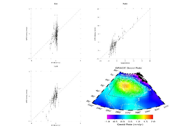
Deformations: GRACE Only vs. GRACE+GPS

GPS Only vs. GRACE+GPS

GRACE and … Radial Only vs. Radial + Horizontals

Conclusions • The GRACE data set can significantly contribute to the GIA field used in SNARF • Observed horizontal velocities don’t significantly alter the derived vertical GIA estimates • When considering only the RMS reduction on of the GPS data, not much difference between ICE 1 and ICE-5 G. However, ICE 5 G does better with the geoid data.

Discussion • How will the product be used? • To that end, how do we define/use/interpret the estimated rotation and translation terms?
- Slides: 20