ASSESSING THE COMBINED IMPACT OF CLIMATE AND LAND

ASSESSING THE COMBINED IMPACT OF CLIMATE AND LAND USE CHANGES ON THE PERFORMANCE OF KANGSABATI IRRIGATION PROJECT Presented by Dhage Pradnya Murlidhar (11 AG 90 J 01) Under the guidance of Prof. N. S. Raghuwanshi Prof. R. Singh Agricultural and Food Engineering Department Indian Institute of Technology Kharagpur

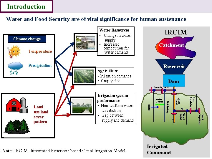
Introduction Water and Food Security are of vital significance for human sustenance Climate change Temperature Water Resources • Change in water supply • Increased competition for water demand IRCIM Catchment Precipitation Reservoir Agriculture • Irrigation demands • Crop yields Dam Branch Canal Cross Regulator Head Regulator Direct Outlet Irrigated Command Main Canal Distributary Note: IRCIM- Integrated Reservoir based Canal Irrigation Model Water Course Outlet Land use land cover pattern Irrigation system performance • Non-uniform water distribution • Gap between supply and demand

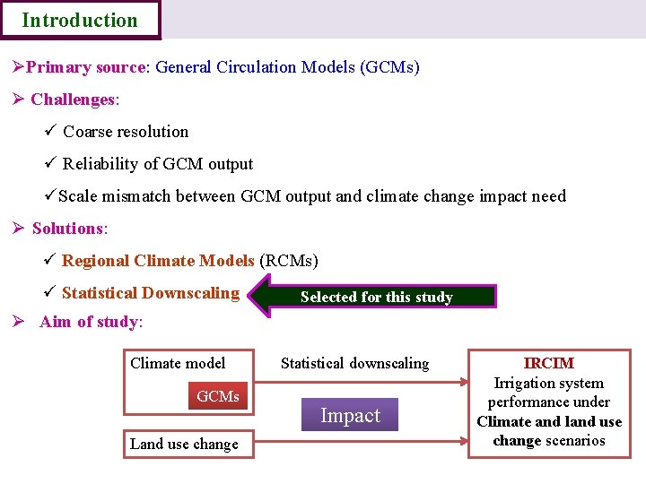
Introduction ØPrimary source: General Circulation Models (GCMs) Ø Challenges: ü Coarse resolution ü Reliability of GCM output üScale mismatch between GCM output and climate change impact need Ø Solutions: ü Regional Climate Models (RCMs) ü Statistical Downscaling Selected for this study Ø Aim of study: Climate model GCMs Land use change Statistical downscaling Impact IRCIM Irrigation system performance under Climate and land use change scenarios

Introduction Data Objectives Methodolo Results gy Conclusion To study the historical performance of Kangsabati irrigation project and to calibrate and validate IRCIM for Kangsabati irrigation project. To develop climate change scenarios at basin scale by statistical downscaling GCM outputs. To study historical land use/land cover pattern and to predict future LU/LC changes using the Cellular Automata (CA)-Markov model. To evaluate the performance of the Kangsabati irrigation project under various plausible climate change scenarios. To study the integrated impact of land use and climate change scenarios on Kangsabati irrigation project performance.

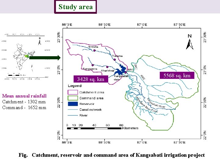
Introduction Study area Methodology Results Conclusion Simulia Tusama Rangagora Kharidwar 3428 sq. km Kangsabati dam 5568 sq. km Mean annual rainfall Catchment - 1302 mm Command - 1652 mm Fig. Catchment, reservoir and command area of Kangsabati irrigation project

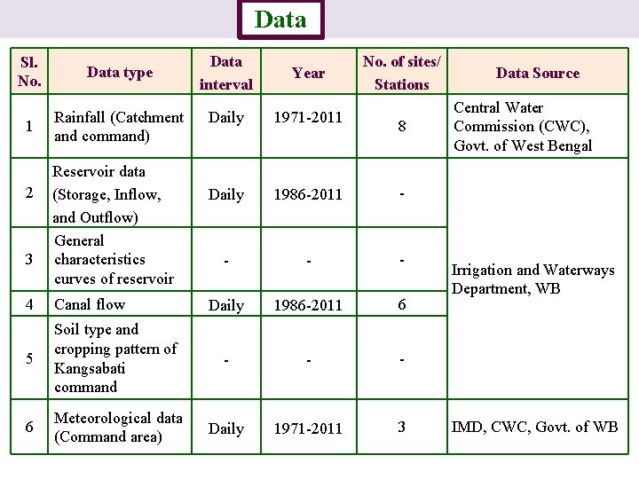
Introduction Sl. No. Data type 1 Rainfall (Catchment and command) 2 3 Data Study area Reservoir data (Storage, Inflow, and Outflow) General characteristics curves of reservoir Methodology Data interval Year No. of sites/ Stations Daily 1971 -2011 Daily 1986 -2011 - - Daily 1986 -2011 6 8 4 Canal flow 5 Soil type and cropping pattern of Kangsabati command - - - 6 Meteorological data (Command area) Daily 1971 -2011 3 Results Conclusion Data Source Central Water Commission (CWC), Govt. of West Bengal Irrigation and Waterways Department, WB IMD, CWC, Govt. of WB

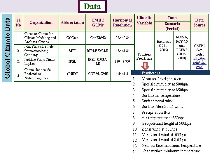
Global Climate Data Introduction Sl. No 1. 2. 3. 4. Study area Organization Canadian Centre for Climate Modeling and Analysis, Canada Max Planck Institute for meteorology, Germany Institute Pierre Simon Laplace Centre National de Recherches Meteorologiques Data Methodology Abbreviation CMIP 5 GCMs Horizontal Resolution CCCma Can. ESM 2 2. 8 o × 2. 8 o MPI-ESM-LR 1. 8 o × 1. 8 o IPSL-CM 5 ALR 1. 9 o × 3. 75 o CNRM-CM 5 1. 4 o × 1. 4 o Results Climatic Variable Data Scenario (Period) Historical (19712005) Fourteen Predictors 1 2 3 4 5 6 7 8 9 10 11 12 13 14 Conclusion RCP 2. 6, RCP 4. 5 and RCP 8. 5 (20062100) Data Source CMIP 5 data portal http: //pc mdi 9. llnl. gov/ Predictors Mean sea level pressure Specific humidity at 500 hpa Specific humidity at 850 hpa Surface air temperature Surface zonal wind Surface Meridional wind Precipitation flux Air temperature at 850 hpa Geopotential height at 500 hpa Zonal wind at 500 hpa Meridional wind at 850 hpa Near surface maximum temperature Near surface minimum temperature

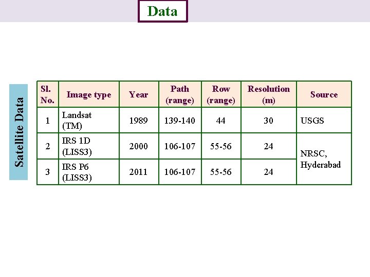
Satellite Data Introduction Sl. No. Study area Image type Data Methodology Results Year Path (range) Row (range) Resolution (m) 1 Landsat (TM) 1989 139 -140 44 30 2 IRS 1 D (LISS 3) 2000 106 -107 55 -56 24 3 IRS P 6 (LISS 3) 2011 106 -107 55 -56 24 Conclusion Source USGS NRSC, Hyderabad

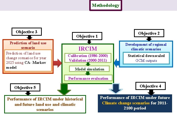
Introduction Study area Objective 3 Prediction of land use scenario Prediction of land use change scenarios for year 2025 using CA- Markov model Data Methodology Results Conclusion Objective 2 Objective 1 IRCIM Development of regional climatic scenarios Calibration (1986 -2000) Validation (2000 -2011) Statistical downscaled GCM outputs Model simulation Performance evaluation Objective 5 Performance of IRCIM under historical and future land use and climatic scenarios Objective 4 Performance of IRCIM under future Climate change scenarios for 20112100 period

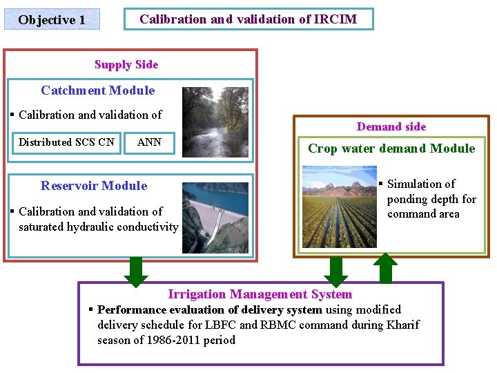
Calibration and validation of IRCIM Objective 1 Supply Side Catchment Module § Calibration and validation of Distributed SCS CN Demand side ANN Crop water demand Module Reservoir Module § Calibration and validation of saturated hydraulic conductivity § Simulation of ponding depth for command area Irrigation Management System § Performance evaluation of delivery system using modified delivery schedule for LBFC and RBMC command during Kharif season of 1986 -2011 period

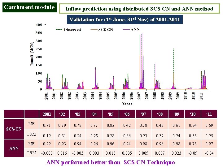
Catchment module Inflow prediction using distributed SCS CN and ANN method Validation for (1 st June- 31 st Nov) of 2001 -2011 2001 ‘ 02 ‘ 03 ‘ 04 ‘ 05 ‘ 06 ‘ 07 ‘ 08 ‘ 09 ‘ 10 ‘ 11 ME 0. 71 0. 79 0. 78 0. 77 0. 82 0. 42 0. 78 0. 48 0. 61 0. 24 0. 69 CRM 0. 19 0. 31 0. 24 0. 25 0. 28 0. 66 0. 23 0. 32 0. 24 0. 33 0. 25 ME 0. 92 0. 93 0. 94 0. 96 0. 94 0. 98 0. 96 0. 98 0. 73 0. 97 CRM -0. 002 0. 016 -0. 003 0. 018 0. 035 0. 005 0. 037 0. 023 -0. 05 -0. 04 SCS-CN ANN performed better than SCS CN Technique

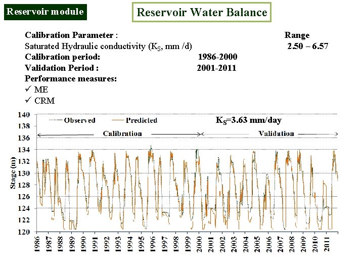
Reservoir module Reservoir Water Balance Calibration Parameter : Range Saturated Hydraulic conductivity (KS, mm /d) 2. 50 – 6. 57 Calibration period: 1986 -2000 Validation Period : 2001 -2011 Performance measures: ü ME ü CRM KS=3. 63 mm/day

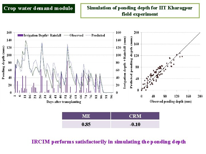
Crop water demand module Simulation of ponding depth for IIT Kharagpur field experiment ME CRM 0. 85 -0. 10 IRCIM performs satisfactorily in simulating the ponding depth

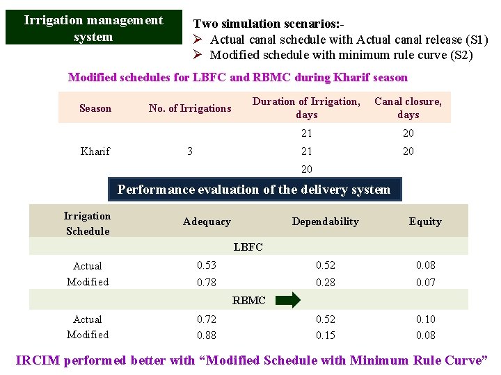
Irrigation management system Two simulation scenarios: Ø Actual canal schedule with Actual canal release (S 1) Ø Modified schedule with minimum rule curve (S 2) Modified schedules for LBFC and RBMC during Kharif season Season Kharif No. of Irrigations Duration of Irrigation, Canal closure, days 3 21 20 20 Performance evaluation of the delivery system Irrigation Schedule Adequacy Dependability Equity 0. 53 0. 52 0. 08 0. 78 0. 28 0. 07 0. 52 0. 15 0. 10 0. 08 LBFC Actual Modified RBMC Actual Modified 0. 72 0. 88 IRCIM performed better with “Modified Schedule with Minimum Rule Curve”

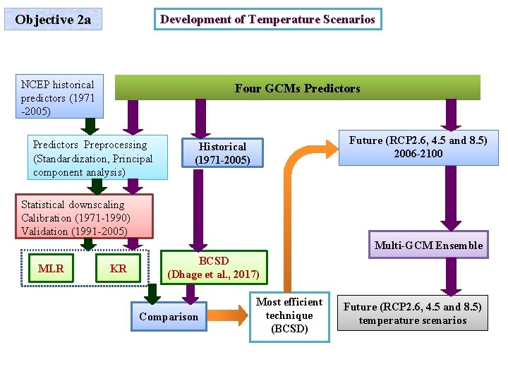
Objective 2 a Development of Temperature Scenarios NCEP historical predictors (1971 -2005) Four GCMs Predictors Preprocessing (Standardization, Principal component analysis) Future (RCP 2. 6, 4. 5 and 8. 5) 2006 -2100 Historical (1971 -2005) Statistical downscaling Calibration (1971 -1990) Validation (1991 -2005) Multi-GCM Ensemble MLR KR BCSD (Dhage et al. , 2017) Comparison Most efficient technique (BCSD) Future (RCP 2. 6, 4. 5 and 8. 5) temperature scenarios

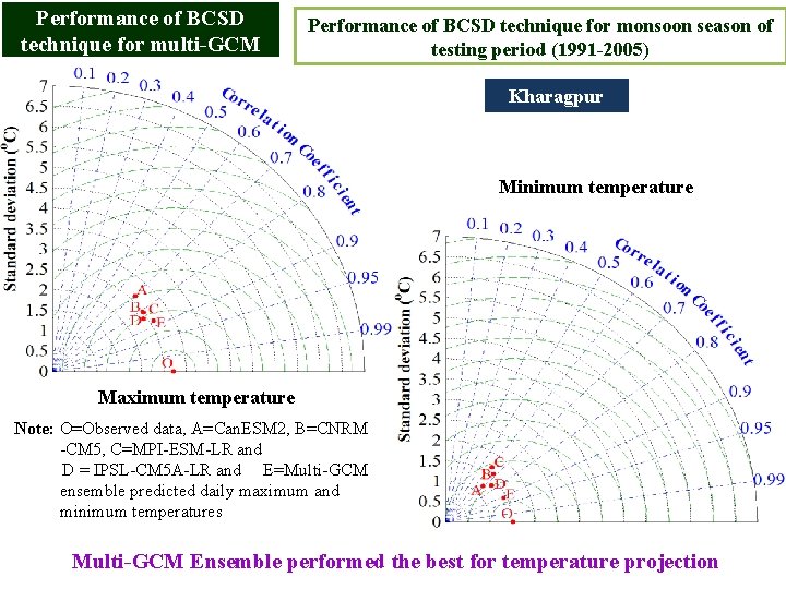
Performance of BCSD technique for multi-GCM Performance of BCSD technique for monsoon season of testing period (1991 -2005) Kharagpur Minimum temperature Maximum temperature Note: O=Observed data, A=Can. ESM 2, B=CNRM -CM 5, C=MPI-ESM-LR and D = IPSL-CM 5 A-LR and E=Multi-GCM ensemble predicted daily maximum and minimum temperatures Multi-GCM Ensemble performed the best for temperature projection

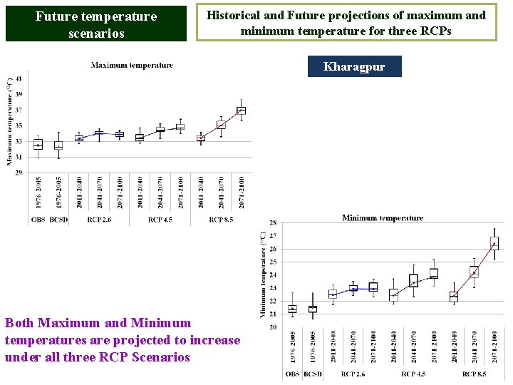
Future temperature scenarios Historical and Future projections of maximum and minimum temperature for three RCPs Kharagpur Both Maximum and Minimum temperatures are projected to increase under all three RCP Scenarios

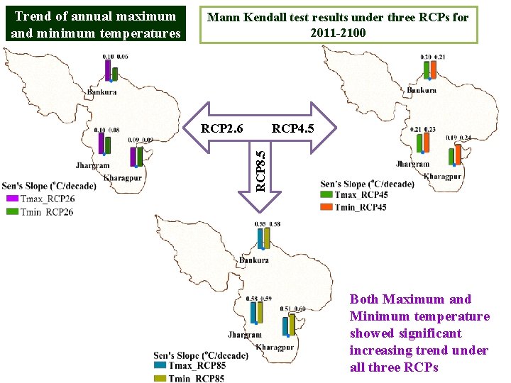
Mann Kendall test results under three RCPs for 2011 -2100 RCP 2. 6 RCP 4. 5 RCP 8. 5 Trend of annual maximum and minimum temperatures Both Maximum and Minimum temperature showed significant increasing trend under all three RCPs

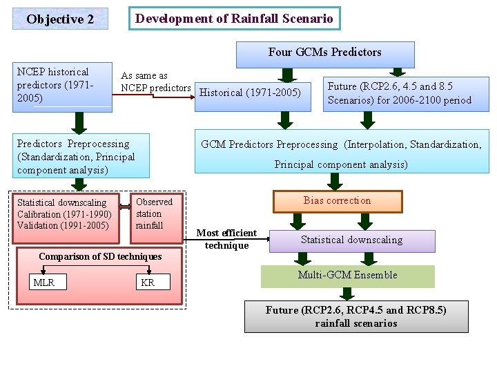
Objective 2 Development of Rainfall Scenario Four GCMs Predictors NCEP historical predictors (19712005) As same as NCEP predictors Historical (1971 -2005) Predictors Preprocessing (Standardization, Principal component analysis) Statistical downscaling Calibration (1971 -1990) Validation (1991 -2005) Future (RCP 2. 6, 4. 5 and 8. 5 Scenarios) for 2006 -2100 period GCM Predictors Preprocessing (Interpolation, Standardization, Principal component analysis) Observed station rainfall Bias correction Most efficient technique Statistical downscaling Comparison of SD techniques MLR KR Multi-GCM Ensemble Future (RCP 2. 6, RCP 4. 5 and RCP 8. 5) rainfall scenarios

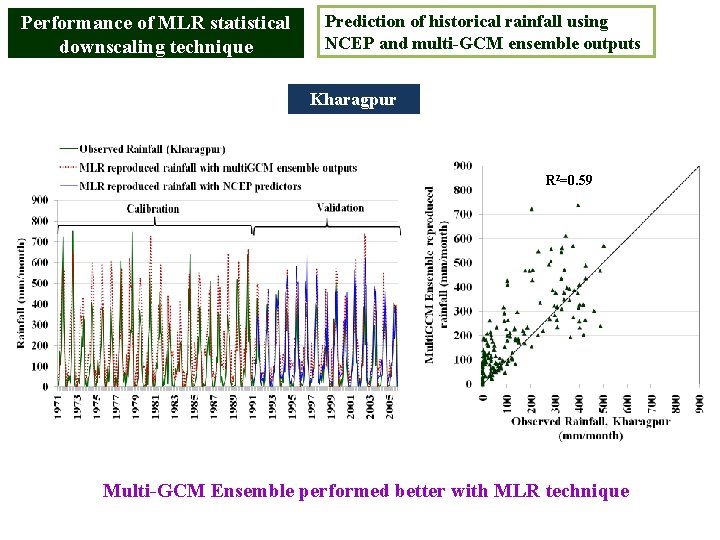
Performance of MLR statistical downscaling technique Prediction of historical rainfall using NCEP and multi-GCM ensemble outputs Kharagpur R 2=0. 59 Multi-GCM Ensemble performed better with MLR technique

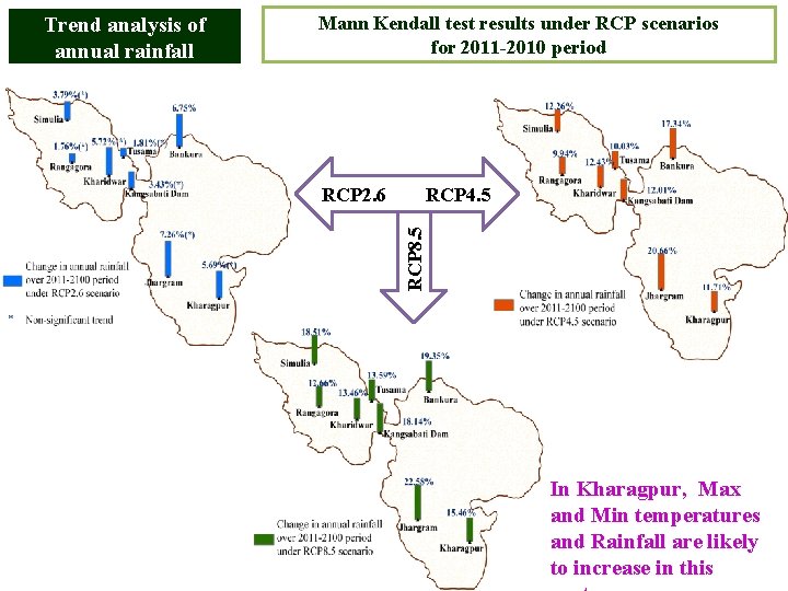
Mann Kendall test results under RCP scenarios for 2011 -2010 period RCP 2. 6 RCP 4. 5 RCP 8. 5 Trend analysis of annual rainfall In Kharagpur, Max and Min temperatures and Rainfall are likely to increase in this

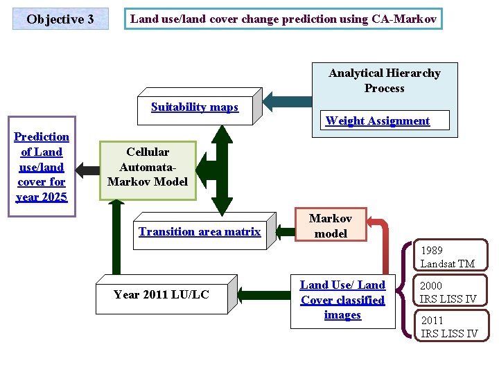
Objective 3 Land use/land cover change prediction using CA-Markov Analytical Hierarchy Process Suitability maps Weight Assignment Prediction of Land use/land cover for year 2025 Cellular Automata. Markov Model Transition area matrix Markov model 1989 Landsat TM Year 2011 LU/LC Land Use/ Land Cover classified images 2000 IRS LISS IV 2011 IRS LISS IV

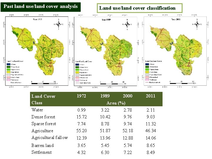
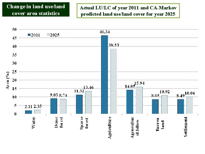
Past land use/land cover analysis Land use/land cover classification Land Cover Class 1972 1989 2000 2011 Water Dense forest Sparse forest Agriculture Agricultural fallow 0. 99 15. 72 7. 74 55. 20 3. 22 10. 42 8. 78 51. 87 2. 78 9. 76 9. 74 52. 18 2. 11 9. 03 11. 32 46. 34 12. 39 13. 96 12. 88 14. 06 Barren land Settlement 3. 65 4. 32 5. 45 6. 30 5. 74 7. 22 8. 65 8. 49 Area (%)

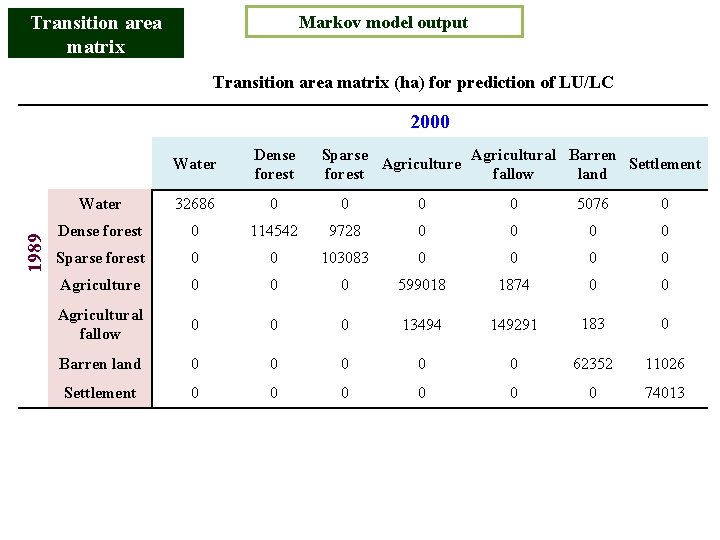
Transition area matrix Markov model output Transition area matrix (ha) for prediction of LU/LC 1989 2000 Water Dense forest Sparse Agricultural Barren Agriculture Settlement forest fallow land Water 32686 0 0 5076 0 Dense forest 0 114542 9728 0 0 Sparse forest 0 0 103083 0 0 Agriculture 0 0 0 599018 1874 0 0 Agricultural fallow 0 0 0 13494 149291 183 0 Barren land 0 0 0 62352 11026 Settlement 0 0 0 74013

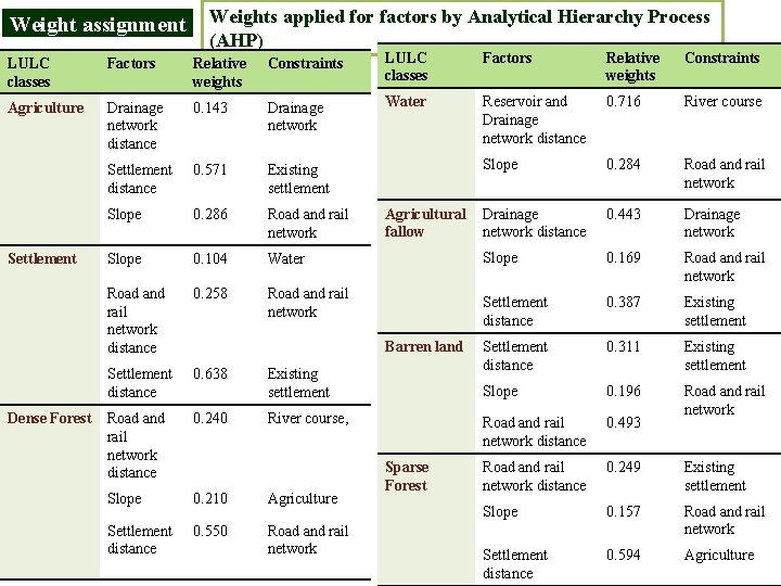
Weight assignment Weights applied for factors by Analytical Hierarchy Process (AHP) LULC classes Factors Relative weights Constraints Agriculture Drainage network distance 0. 143 Drainage network Water Reservoir and Drainage network distance 0. 716 River course Settlement distance 0. 571 Existing settlement Slope 0. 284 Road and rail network Slope 0. 286 Road and rail network 0. 443 Drainage network Slope 0. 104 Water Slope 0. 169 Road and rail network distance 0. 258 Road and rail network Settlement distance 0. 387 Existing settlement 0. 311 Settlement distance 0. 638 Settlement distance Existing settlement Slope 0. 196 Road and rail network distance 0. 240 Road and rail network distance 0. 493 Road and rail network 0. 249 Slope 0. 210 Agriculture Road and rail network distance Existing settlement Slope 0. 157 Settlement distance 0. 550 Road and rail network Settlement distance 0. 594 Agriculture Settlement Dense Forest Agricultural Drainage fallow network distance Barren land Existing settlement River course, Sparse Forest

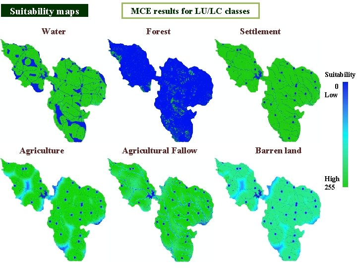
Suitability maps Water MCE results for LU/LC classes Forest Settlement Suitability 0 Low Agriculture Agricultural Fallow Barren land High 255

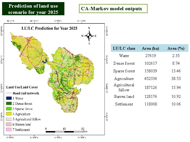
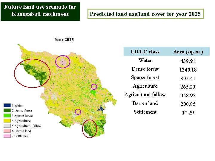
Prediction of land use scenario for year 2025 CA-Markov model outputs LU/LC class Area (ha) Area (%) Water 27619 2. 35 Dense forest 102617 8. 74 Sparse forest 158039 13. 46 Agriculture 452336 38. 53 Agricultural fallow 187126 15. 94 Barren land 128176 10. 92 Settlement 118008 10. 06

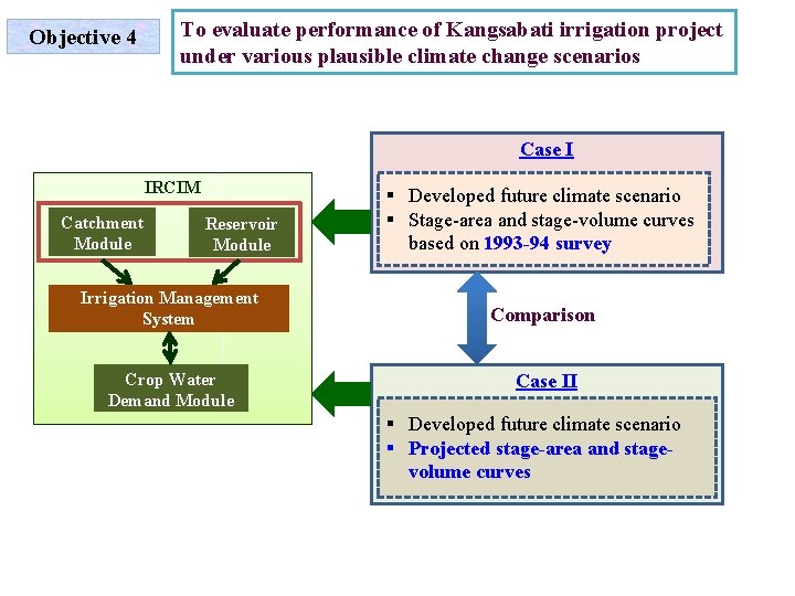
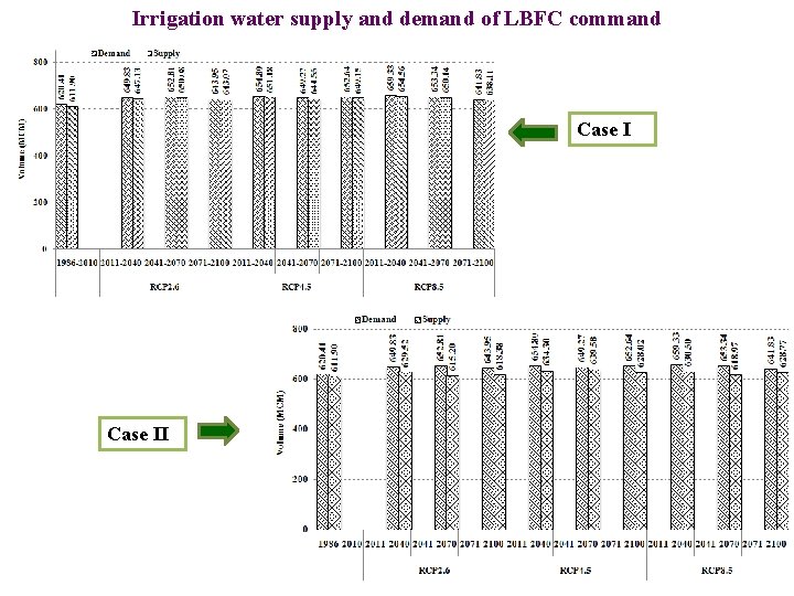
To evaluate performance of Kangsabati irrigation project under various plausible climate change scenarios Objective 4 Case I IRCIM Catchment Module Reservoir Module Irrigation Management System Crop Water Demand Module § Developed future climate scenario § Stage-area and stage-volume curves based on 1993 -94 survey Comparison Case II § Developed future climate scenario § Projected stage-area and stagevolume curves

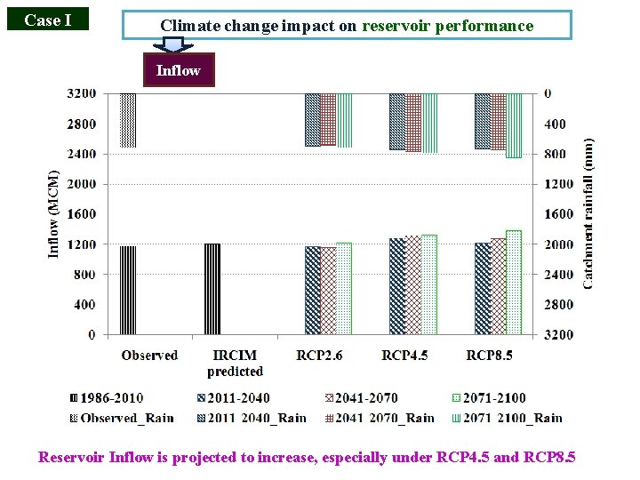
Case I Climate change impact on reservoir performance Inflow Reservoir Inflow is projected to increase, especially under RCP 4. 5 and RCP 8. 5

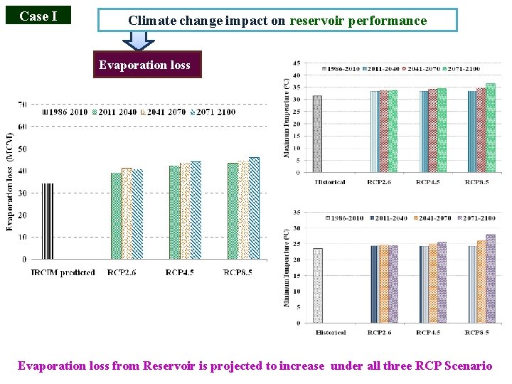
Case I Climate change impact on reservoir performance Evaporation loss from Reservoir is projected to increase under all three RCP Scenario

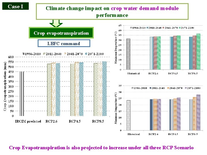
Case I Climate change impact on crop water demand module performance Crop evapotranspiration LBFC command Crop Evapotranspiration is also projected to increase under all three RCP Scenario

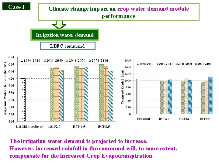
Case I Climate change impact on crop water demand module performance Irrigation water demand LBFC command The irrigation water demand is projected to increase. However, increased rainfall in the command will, to some extent, compensate for the increased Crop Evapotranspiration

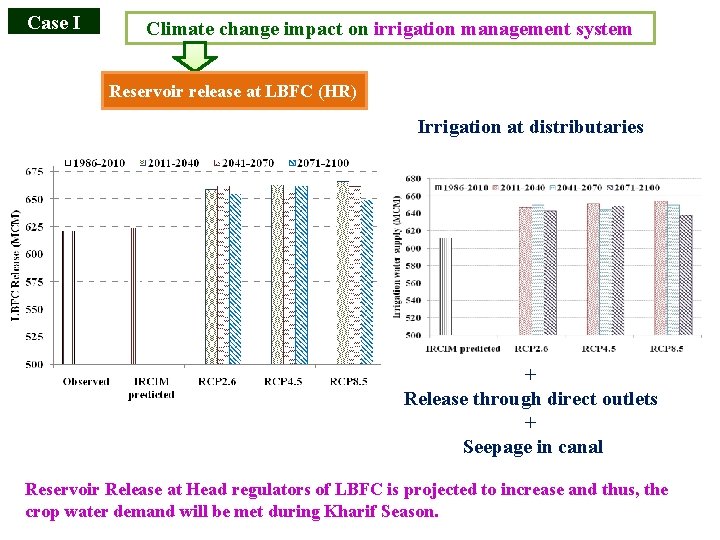
Case I Climate change impact on irrigation management system Reservoir release at LBFC (HR) Irrigation at distributaries + Release through direct outlets + Seepage in canal Reservoir Release at Head regulators of LBFC is projected to increase and thus, the crop water demand will be met during Kharif Season.

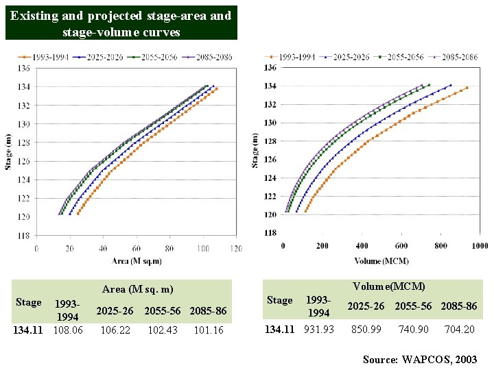
Existing and projected stage-area and stage-volume curves Volume(MCM) Area (M sq. m) Stage 19931994 134. 11 108. 06 2025 -26 2055 -56 2085 -86 106. 22 102. 43 101. 16 19931994 134. 11 931. 93 Stage 2025 -26 2055 -56 2085 -86 850. 99 740. 90 704. 20 Source: WAPCOS, 2003

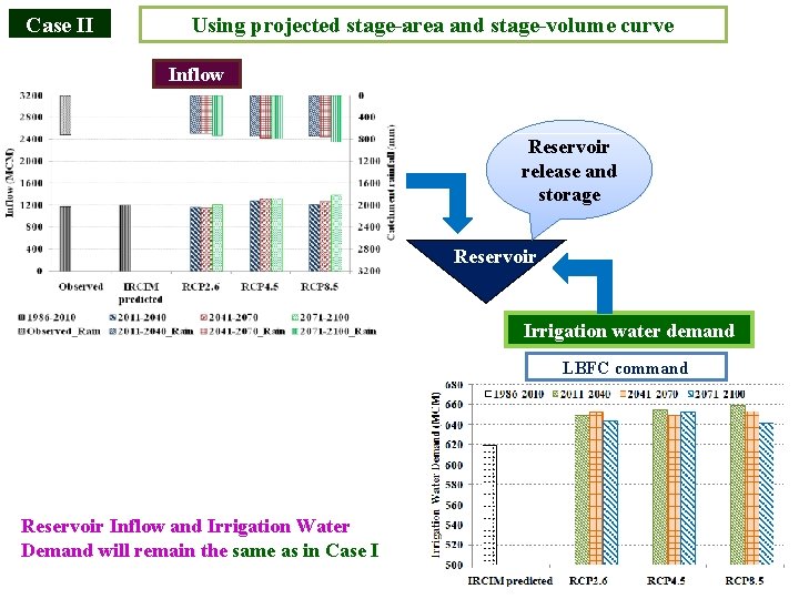
Case II Using projected stage-area and stage-volume curve Inflow Reservoir release and storage Reservoir Irrigation water demand LBFC command Reservoir Inflow and Irrigation Water Demand will remain the same as in Case I

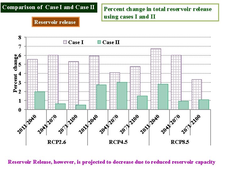
Comparison of Case I and Case II Percent change in total reservoir release using cases I and II Reservoir release 8 Case I Percent change 7 Case II 6 5 4 3 2 1 RCP 2. 6 RCP 4. 5 -2 10 20 71 20 7 41 20 0 20 11 - 20 4 0 20 71 - 21 0 0 41 - 20 20 4 11 20 20 7 0 0 20 71 - 21 0 0 20 7 41 - 20 20 11 - 20 4 0 0 RCP 8. 5 Reservoir Release, however, is projected to decrease due to reduced reservoir capacity

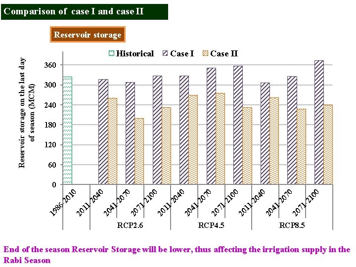
Comparison of case I and case II Reservoir storage on the last day of season (MCM) Reservoir storage Historical Case II 360 300 240 180 120 60 RCP 2. 6 20 11 -2 04 0 20 41 -2 07 0 20 71 -2 10 0 21 00 71 - 20 20 70 41 - 20 20 11 - 20 40 21 00 71 - 20 20 70 41 - 20 20 40 11 - 20 19 86 - 20 10 0 RCP 4. 5 RCP 8. 5 End of the season Reservoir Storage will be lower, thus affecting the irrigation supply in the Rabi Season

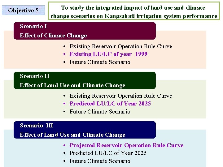
Objective 5 To study the integrated impact of land use and climate change scenarios on Kangsabati irrigation system performance Scenario I Effect of Climate Change • Existing Reservoir Operation Rule Curve • Existing LU/LC of year 1999 • Future Climate Scenario II Effect of Land Use and Climate Change • Existing Reservoir Operation Rule Curve • Predicted LU/LC of Year 2025 • Future Climate Scenario III Effect of Land Use and Climate Change • Projected Reservoir Operation Rule Curve • Predicted LU/LC of Year 2025 • Future Climate Scenario

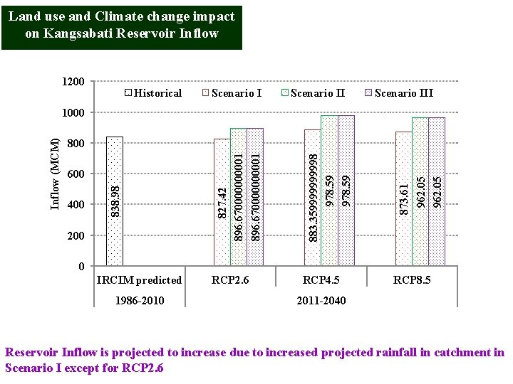
Land use and Climate change impact on Kangsabati Reservoir Inflow 1200 Historical Scenario III 200 873. 61 962. 05 400 883. 35999998 978. 59 600 827. 42 896. 670000000001 800 838. 98 Inflow (MCM) 1000 0 IRCIM predicted 1986 -2010 RCP 2. 6 RCP 4. 5 RCP 8. 5 2011 -2040 Reservoir Inflow is projected to increase due to increased projected rainfall in catchment in Scenario I except for RCP 2. 6

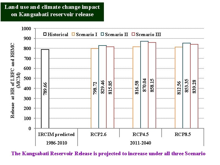
Land use and climate change impact on Kangsabati reservoir release 1000 Historical Scenario III 800 700 839. 28 853. 35 812. 56 858. 15 870. 04 816. 58 815. 85 400 798. 72 500 829. 46 600 789. 66 Release at HR of LBFC and RBMC (MCM) 900 300 200 100 0 IRCIM predicted 1986 -2010 RCP 2. 6 RCP 4. 5 RCP 8. 5 2011 -2040 The Kangsabati Reservoir Release is projected to increase under all three Scenario

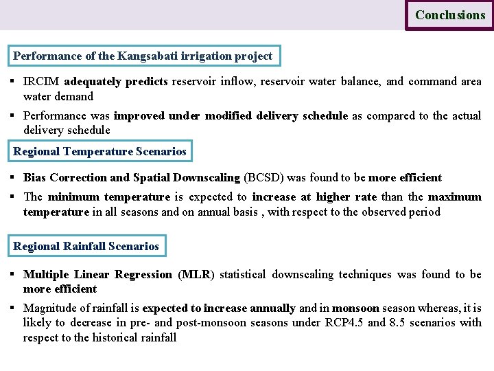
Introduction Study area Data Methodology Results Conclusions Performance of the Kangsabati irrigation project § IRCIM adequately predicts reservoir inflow, reservoir water balance, and command area water demand § Performance was improved under modified delivery schedule as compared to the actual delivery schedule Regional Temperature Scenarios § Bias Correction and Spatial Downscaling (BCSD) was found to be more efficient § The minimum temperature is expected to increase at higher rate than the maximum temperature in all seasons and on annual basis , with respect to the observed period Regional Rainfall Scenarios § Multiple Linear Regression (MLR) statistical downscaling techniques was found to be more efficient § Magnitude of rainfall is expected to increase annually and in monsoon season whereas, it is likely to decrease in pre- and post-monsoon seasons under RCP 4. 5 and 8. 5 scenarios with respect to the historical rainfall

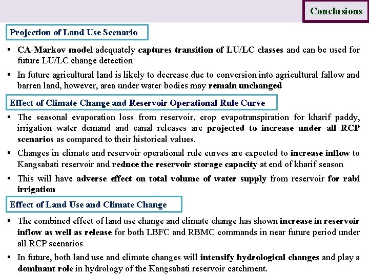
Introduction Study area Data Methodology Results Conclusions Projection of Land Use Scenario § CA-Markov model adequately captures transition of LU/LC classes and can be used for future LU/LC change detection § In future agricultural land is likely to decrease due to conversion into agricultural fallow and barren land, however, area under water bodies may remain unchanged Effect of Climate Change and Reservoir Operational Rule Curve § The seasonal evaporation loss from reservoir, crop evapotranspiration for kharif paddy, irrigation water demand canal releases are projected to increase under all RCP scenarios as compared to their historical values. § Changes in climate and reservoir operational rule curves are expected to increase inflow to Kangsabati reservoir and reduce the reservoir storage capacity at end of kharif season § This will have adverse effect on total volume of water supply from reservoir for rabi irrigation Effect of Land Use and Climate Change § The combined effect of land use change and climate change has shown increase in reservoir inflow as well as release for both LBFC and RBMC commands in near future period under all RCP scenarios § In future, both land use and climate changes will intensify hydrological changes and play a dominant role in hydrology of the Kangsabati reservoir catchment.

Research contributions The best statistical downscaling techniques for rainfall and temperature projections were identified. Multi-GCM Ensemble Outputs were statistically downscaled to develop the climate change scenarios under RCP 2. 6, 4. 5 and 8. 5 CA-Markov model was used for predicting the Land Use change in the near future period. The Integrated Impact of Climate and Land Use Changes on irrigation system performance of a reservoir-based irrigation project was investigated.

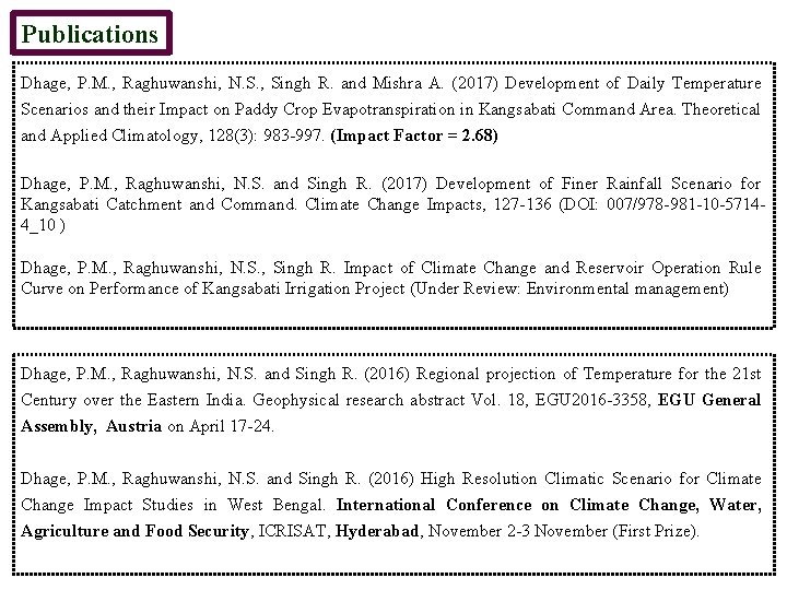
Publications Dhage, P. M. , Raghuwanshi, N. S. , Singh R. and Mishra A. (2017) Development of Daily Temperature Scenarios and their Impact on Paddy Crop Evapotranspiration in Kangsabati Command Area. Theoretical and Applied Climatology, 128(3): 983 -997. (Impact Factor = 2. 68) Dhage, P. M. , Raghuwanshi, N. S. and Singh R. (2017) Development of Finer Rainfall Scenario for Kangsabati Catchment and Command. Climate Change Impacts, 127 -136 (DOI: 007/978 -981 -10 -57144_10 ) Dhage, P. M. , Raghuwanshi, N. S. , Singh R. Impact of Climate Change and Reservoir Operation Rule Curve on Performance of Kangsabati Irrigation Project (Under Review: Environmental management) Dhage, P. M. , Raghuwanshi, N. S. and Singh R. (2016) Regional projection of Temperature for the 21 st Century over the Eastern India. Geophysical research abstract Vol. 18, EGU 2016 -3358, EGU General Assembly, Austria on April 17 -24. Dhage, P. M. , Raghuwanshi, N. S. and Singh R. (2016) High Resolution Climatic Scenario for Climate Change Impact Studies in West Bengal. International Conference on Climate Change, Water, Agriculture and Food Security, ICRISAT, Hyderabad, November 2 -3 November (First Prize).

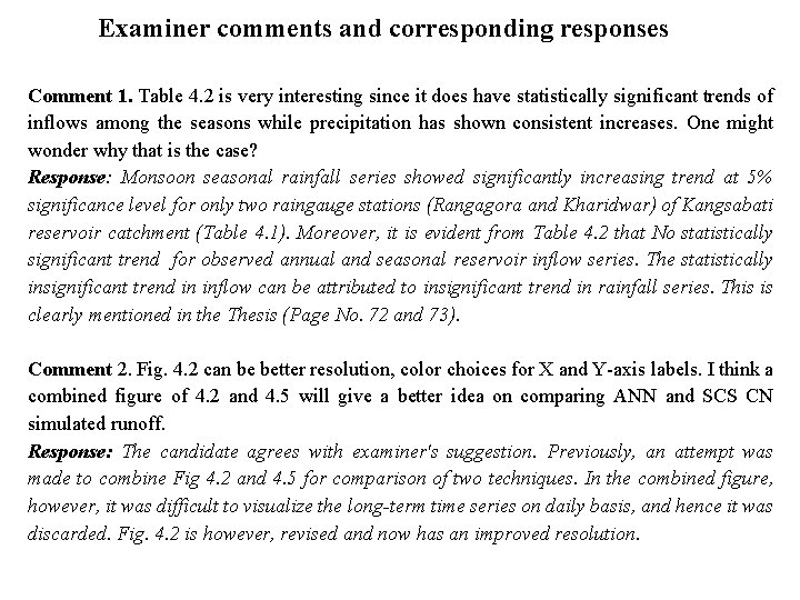
Examiner comments and corresponding responses Comment 1. Table 4. 2 is very interesting since it does have statistically significant trends of inflows among the seasons while precipitation has shown consistent increases. One might wonder why that is the case? Response: Monsoon seasonal rainfall series showed significantly increasing trend at 5% significance level for only two raingauge stations (Rangagora and Kharidwar) of Kangsabati reservoir catchment (Table 4. 1). Moreover, it is evident from Table 4. 2 that No statistically significant trend for observed annual and seasonal reservoir inflow series. The statistically insignificant trend in inflow can be attributed to insignificant trend in rainfall series. This is clearly mentioned in the Thesis (Page No. 72 and 73). Comment 2. Fig. 4. 2 can be better resolution, color choices for X and Y-axis labels. I think a combined figure of 4. 2 and 4. 5 will give a better idea on comparing ANN and SCS CN simulated runoff. Response: The candidate agrees with examiner's suggestion. Previously, an attempt was made to combine Fig 4. 2 and 4. 5 for comparison of two techniques. In the combined figure, however, it was difficult to visualize the long-term time series on daily basis, and hence it was discarded. Fig. 4. 2 is however, revised and now has an improved resolution.

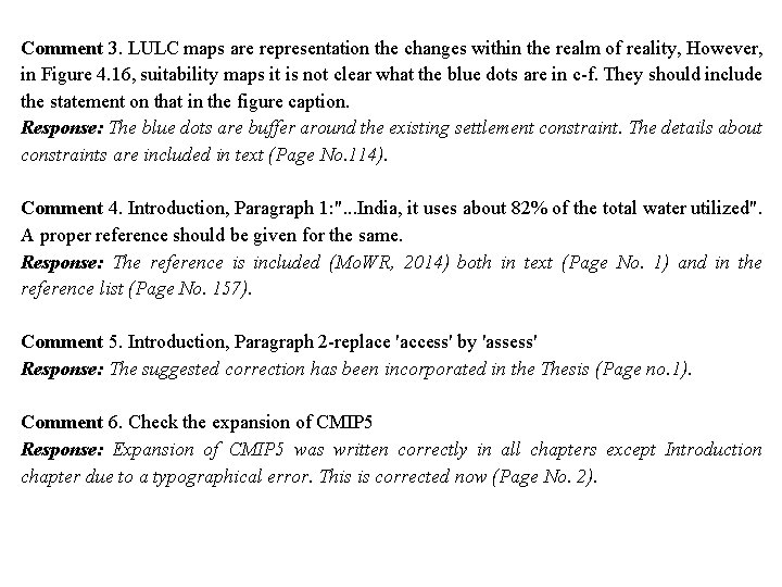
Comment 3. LULC maps are representation the changes within the realm of reality, However, in Figure 4. 16, suitability maps it is not clear what the blue dots are in c-f. They should include the statement on that in the figure caption. Response: The blue dots are buffer around the existing settlement constraint. The details about constraints are included in text (Page No. 114). Comment 4. Introduction, Paragraph 1: ". . . India, it uses about 82% of the total water utilized". A proper reference should be given for the same. Response: The reference is included (Mo. WR, 2014) both in text (Page No. 1) and in the reference list (Page No. 157). Comment 5. Introduction, Paragraph 2 -replace 'access' by 'assess' Response: The suggested correction has been incorporated in the Thesis (Page no. 1). Comment 6. Check the expansion of CMIP 5 Response: Expansion of CMIP 5 was written correctly in all chapters except Introduction chapter due to a typographical error. This is corrected now (Page No. 2).

Comment 7. Expansion of GCM- Is it ' Global Climate Model' or 'General Circulation Model'? Response: In IPCC AR 4 report uses the term Global climate model (GCM, but IPCC AR 5 report states that "Global climate model" refer to an integrated framework that incorporates multiple components including a General Circulation Model. Since an integrated framework for downscaling not used here, the GCM expansion is changed to "General Circulation Model" in thesis. Comment 8. Introduction, Paragraph 5 - Sachindra et al. 2014 c- this is appearing for the first time so should be 2014 a. Response: The error is corrected (Pages No. 2 and 159). In addition to above, thesis has been carefully revised to take care of grammatical and typographical errors, if any. The candidate is thankful to both examiners for their helpful comments and suggestions.

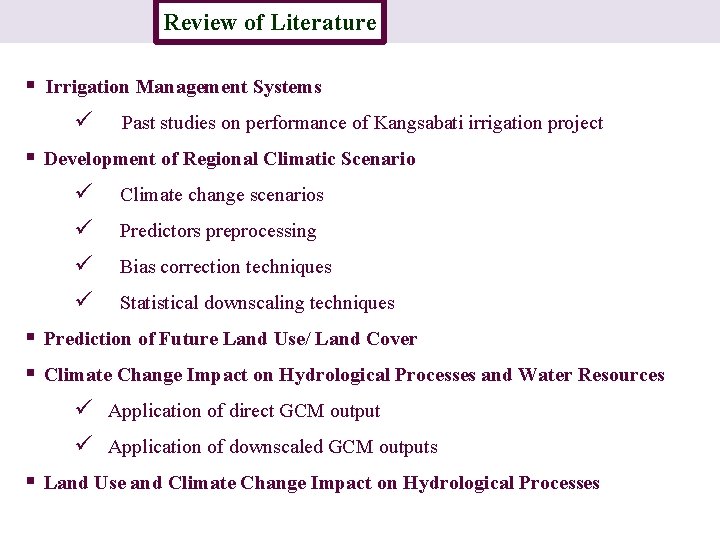
Review of Literature Introduction § Irrigation Management Systems ü Past studies on performance of Kangsabati irrigation project § Development of Regional Climatic Scenario ü Climate change scenarios ü Predictors preprocessing ü Bias correction techniques ü Statistical downscaling techniques § Prediction of Future Land Use/ Land Cover § Climate Change Impact on Hydrological Processes and Water Resources ü Application of direct GCM output ü Application of downscaled GCM outputs § Land Use and Climate Change Impact on Hydrological Processes

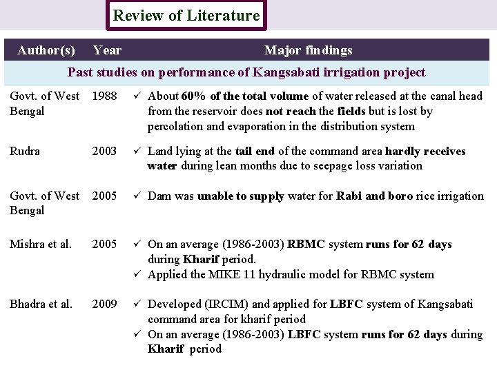
Review of Literature Introduction Author(s) Year Major findings Past studies on performance of Kangsabati irrigation project Govt. of West 1988 Bengal ü About 60% of the total volume of water released at the canal head from the reservoir does not reach the fields but is lost by percolation and evaporation in the distribution system Rudra 2003 ü Land lying at the tail end of the command area hardly receives water during lean months due to seepage loss variation Govt. of West 2005 Bengal ü Dam was unable to supply water for Rabi and boro rice irrigation Mishra et al. 2005 ü Bhadra et al. 2009 ü On an average (1986 -2003) RBMC system runs for 62 days during Kharif period. ü Applied the MIKE 11 hydraulic model for RBMC system Developed (IRCIM) and applied for LBFC system of Kangsabati command area for kharif period ü On an average (1986 -2003) LBFC system runs for 62 days during Kharif period

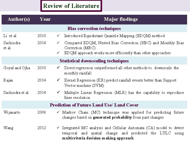
Review of Literature Introduction Author(s) Year Major findings Bias correction techniques Li et al. 2010 ü Introduced Equidistant Quantile Mapping (EDQM) method Sachindra et al. 2014 ü Compared EDQM, Nested Bias Correction (NBC) and Monthly Bias Correction (MBC) EDQM approach works more efficiently than other approaches ü Statistical downscaling techniques Goyal and Ojha 2010 ü Direct regression outperformed all other methods to downscale the monthly rainfall Rajan 2014 ü Kernel Regression (KR) predict rainfall events better than Support Vector machine (SVM) Sachindra et al. 2014 ü Multiple Linear Regression (MLR) has the capability to reproduce finer resolution Prediction of Future Land Use/ Land Cover Wijanarto 2006 ü Markov Chain (MC) technique was applied for predicting future changes based on generated probability from past changes Wang 2012 ü Integrated MC analysis and Cellular Automata (CA) model to detect temporal and spatial change and predicted the LULC using multicriteria decision making approach

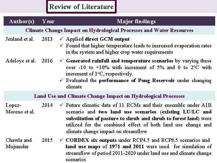
Review of Literature Introduction Author(s) Year Major findings Climate Change Impact on Hydrological Processes and Water Resources Jeuland et al. 2013 ü ü Adeloye et al. 2016 ü Applied direct GCM output Found that higher temperature leads to increased evaporation rates in the system and higher crop water requirements Generated rainfall and temperature scenarios by varying these over -10 to +10% with increment of 5% and 0 to 2 o. C with increment of 1 o. C, respectively. ü Evaluated the performance of Pong Reservoir under changing climate Land Use and Climate Change Impact on Hydrological Processes Lopez. Moreno et al. 2014 ü Future climatic data of 11 RCMs and their ensemble under A 1 B scenario and two land use scenarios (existing LU/LC and substitution of pasture to shrub and shrub to forest land) were utilized for the combined effect of both land use change and climate change impact on streamflow Chawla and Mujumdar 2015 ü CORDEX six outputs under RCP 4. 5 and RCP 8. 5 scenarios and land use maps of 1971 and 2011 were used for simulation of streamflow of period 2011 -2020 under land use and climate change scenarios

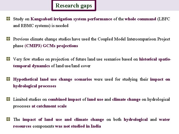
Research gaps Introduction Study on Kangsabati irrigation system performance of the whole command (LBFC and RBMC systems) is needed Previous climate change studies have used the Coupled Model Intercomparison Project phase (CMIP 3) GCMs projections Very few studies on projection of future land use scenarios based on historical spatiotemporal dynamics of land use/land cover Hypothetical land use change scenarios were used for studying their impact on hydrological processes Limited studies on combined impact of land use and climate change on hydrological processes at catchment scale The impact of land use and climate change on both hydrological and water resources components was not studied in India

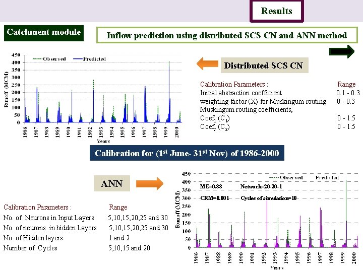
Introduction Catchment module Study area Data Methodology Results Conclusion Inflow prediction using distributed SCS CN and ANN method Distributed SCS CN Calibration Parameters : Range Initial abstraction coefficient 0. 1 - 0. 3 weighting factor (X) for Muskingum routing 0 - 0. 3 Muskingum routing coefficients, Coef 1 (C 1) 0 - 1. 5 Coef 2 (C 2) 0 - 1. 5 Calibration for (1 st June- 31 st Nov) of 1986 -2000 ANN Calibration Parameters : Range No. of Neurons in Input Layers 5, 10, 15, 20, 25 and 30 No. of neurons in hidden Layers 5, 10, 15, 20, 25 and 30 No. of Hidden layers 1 and 2 Number of Cycles 5, 10, 15 and 20 ME=0. 88 Network=20 -20 -1 CRM=0. 001 Cycles of simulation=10

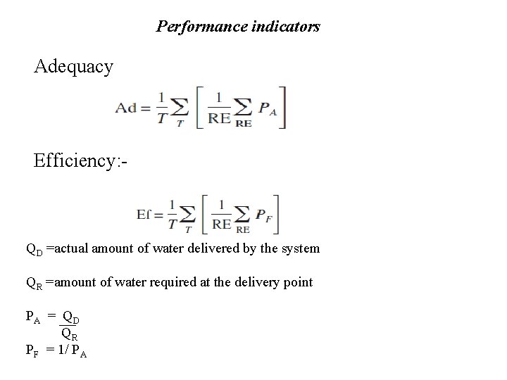
Performance indicators Adequacy Efficiency: - QD =actual amount of water delivered by the system QR =amount of water required at the delivery point PA = QD QR PF = 1/ PA

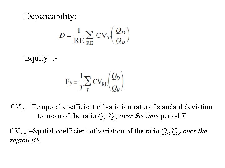
Dependability: - Equity : - CVT = Temporal coefficient of variation ratio of standard deviation to mean of the ratio QD/QR over the time period T CVRE =Spatial coefficient of variation of the ratio QD/QR over the region RE.

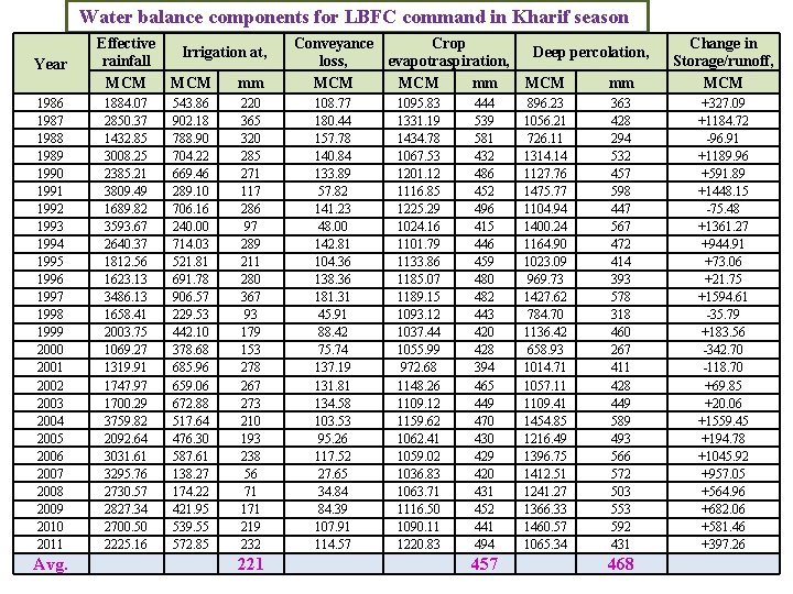
Water balance components for LBFC command in Kharif season Year 1986 1987 1988 1989 1990 1991 1992 1993 1994 1995 1996 1997 1998 1999 2000 2001 2002 2003 2004 2005 2006 2007 2008 2009 2010 2011 Avg. Effective Irrigation at, rainfall MCM mm 1884. 07 2850. 37 1432. 85 3008. 25 2385. 21 3809. 49 1689. 82 3593. 67 2640. 37 1812. 56 1623. 13 3486. 13 1658. 41 2003. 75 1069. 27 1319. 91 1747. 97 1700. 29 3759. 82 2092. 64 3031. 61 3295. 76 2730. 57 2827. 34 2700. 50 2225. 16 543. 86 902. 18 788. 90 704. 22 669. 46 289. 10 706. 16 240. 00 714. 03 521. 81 691. 78 906. 57 229. 53 442. 10 378. 68 685. 96 659. 06 672. 88 517. 64 476. 30 587. 61 138. 27 174. 22 421. 95 539. 55 572. 85 220 365 320 285 271 117 286 97 289 211 280 367 93 179 153 278 267 273 210 193 238 56 71 171 219 232 221 Conveyance Crop loss, evapotraspiration, MCM mm 108. 77 180. 44 157. 78 140. 84 133. 89 57. 82 141. 23 48. 00 142. 81 104. 36 138. 36 181. 31 45. 91 88. 42 75. 74 137. 19 131. 81 134. 58 103. 53 95. 26 117. 52 27. 65 34. 84 84. 39 107. 91 114. 57 1095. 83 1331. 19 1434. 78 1067. 53 1201. 12 1116. 85 1225. 29 1024. 16 1101. 79 1133. 86 1185. 07 1189. 15 1093. 12 1037. 44 1055. 99 972. 68 1148. 26 1109. 12 1159. 62 1062. 41 1059. 02 1036. 83 1063. 71 1116. 50 1090. 11 1220. 83 444 539 581 432 486 452 496 415 446 459 480 482 443 420 428 394 465 449 470 430 429 420 431 452 441 494 457 MCM mm Change in Storage/runoff, MCM 896. 23 1056. 21 726. 11 1314. 14 1127. 76 1475. 77 1104. 94 1400. 24 1164. 90 1023. 09 969. 73 1427. 62 784. 70 1136. 42 658. 93 1014. 71 1057. 11 1109. 41 1454. 85 1216. 49 1396. 75 1412. 51 1241. 27 1366. 33 1460. 57 1065. 34 363 428 294 532 457 598 447 567 472 414 393 578 318 460 267 411 428 449 589 493 566 572 503 553 592 431 +327. 09 +1184. 72 -96. 91 +1189. 96 +591. 89 +1448. 15 -75. 48 +1361. 27 +944. 91 +73. 06 +21. 75 +1594. 61 -35. 79 +183. 56 -342. 70 -118. 70 +69. 85 +20. 06 +1559. 45 +194. 78 +1045. 92 +957. 05 +564. 96 +682. 06 +581. 46 +397. 26 Deep percolation, 468

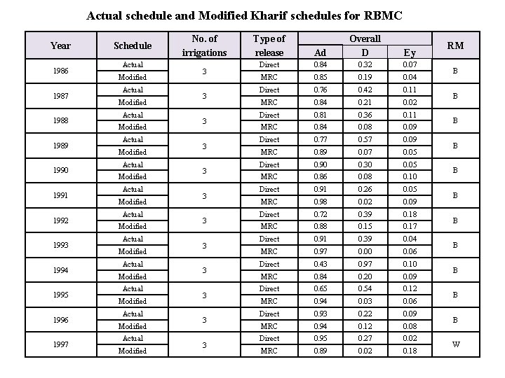
Actual schedule and Modified Kharif schedules for RBMC Year 1986 1987 1988 1989 1990 1991 1992 1993 1994 1995 1996 1997 Schedule Actual Modified Actual Modified Actual Modified No. of irrigations 3 3 3 Type of release Ad Overall D Ey Direct 0. 84 0. 32 0. 07 MRC 0. 85 0. 19 0. 04 Direct 0. 76 0. 42 0. 11 MRC 0. 84 0. 21 0. 02 Direct 0. 81 0. 36 0. 11 MRC 0. 84 0. 08 0. 09 Direct 0. 77 0. 57 0. 09 MRC 0. 89 0. 07 0. 05 Direct 0. 90 0. 30 0. 05 MRC 0. 86 0. 08 0. 10 Direct 0. 91 0. 26 0. 05 MRC 0. 98 0. 02 0. 09 Direct 0. 72 0. 39 0. 18 MRC 0. 88 0. 15 0. 17 Direct 0. 91 0. 39 0. 04 MRC 0. 97 0. 00 0. 06 Direct 0. 43 0. 97 0. 10 MRC 0. 84 0. 20 0. 09 Direct 0. 65 0. 54 0. 12 MRC 0. 94 0. 03 0. 06 Direct 0. 93 0. 22 0. 09 MRC 0. 94 0. 12 0. 08 Direct 0. 95 0. 27 0. 02 MRC 0. 89 0. 02 0. 18 RM B B B W

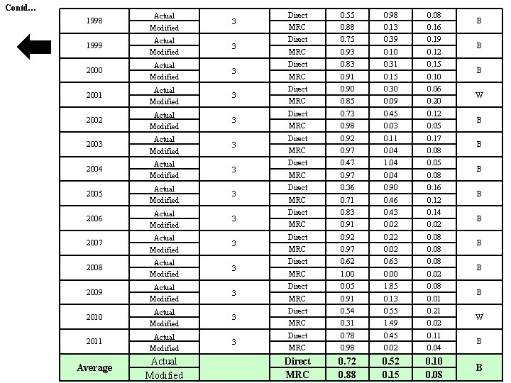
Contd… 1998 Actual Modified 3 1999 Actual Modified 3 2000 Actual Modified 3 2001 Actual Modified 3 2002 Actual Modified 3 2003 Actual Modified 3 2004 Actual Modified 3 2005 Actual Modified 3 2006 Actual Modified 3 2007 Actual Modified 3 2008 Actual Modified 3 2009 Actual Modified 3 2010 Actual Modified 3 2011 Actual Modified 3 Average Actual Modified Direct 0. 55 0. 98 0. 08 MRC 0. 88 0. 13 0. 16 Direct 0. 75 0. 39 0. 19 MRC 0. 93 0. 10 0. 12 Direct 0. 83 0. 31 0. 15 MRC 0. 91 0. 15 0. 10 Direct 0. 90 0. 30 0. 06 MRC 0. 85 0. 09 0. 20 Direct 0. 73 0. 45 0. 12 MRC 0. 98 0. 03 0. 05 Direct 0. 92 0. 11 0. 17 MRC 0. 97 0. 04 0. 08 Direct 0. 47 1. 04 0. 05 MRC 0. 97 0. 04 0. 08 Direct 0. 36 0. 90 0. 16 MRC 0. 71 0. 46 0. 12 Direct 0. 83 0. 43 0. 14 MRC 0. 91 0. 02 Direct 0. 92 0. 22 0. 08 MRC 0. 97 0. 02 0. 08 Direct 0. 62 0. 63 0. 08 MRC 1. 00 0. 02 Direct 0. 05 1. 85 0. 08 MRC 0. 91 0. 13 0. 01 Direct 0. 54 0. 55 0. 21 MRC 0. 31 1. 49 0. 02 Direct 0. 78 0. 45 0. 11 MRC 0. 98 0. 02 0. 04 Direct MRC 0. 72 0. 88 0. 52 0. 15 0. 10 0. 08 B B B W B B

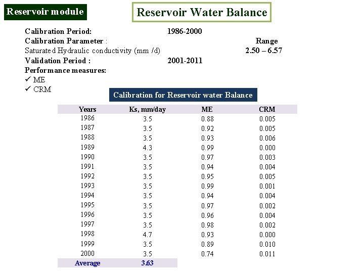
Reservoir module Reservoir Water Balance Calibration Period: 1986 -2000 Calibration Parameter : Range Saturated Hydraulic conductivity (mm /d) 2. 50 – 6. 57 Validation Period : 2001 -2011 Performance measures: ü ME ü CRM Calibration for Reservoir water Balance Years 1986 1987 1988 1989 1990 1991 1992 1993 1994 1995 1996 1997 1998 1999 2000 Average Ks, mm/day 3. 5 4. 3 3. 5 3. 5 4. 7 3. 5 3. 63 ME 0. 88 0. 92 0. 93 0. 99 0. 97 0. 94 0. 95 0. 99 0. 94 0. 97 0. 96 0. 98 0. 93 0. 89 0. 74 CRM 0. 005 0. 006 0. 000 0. 003 0. 004 0. 005 0. 001 0. 004 0. 002 0. 000 0. 011

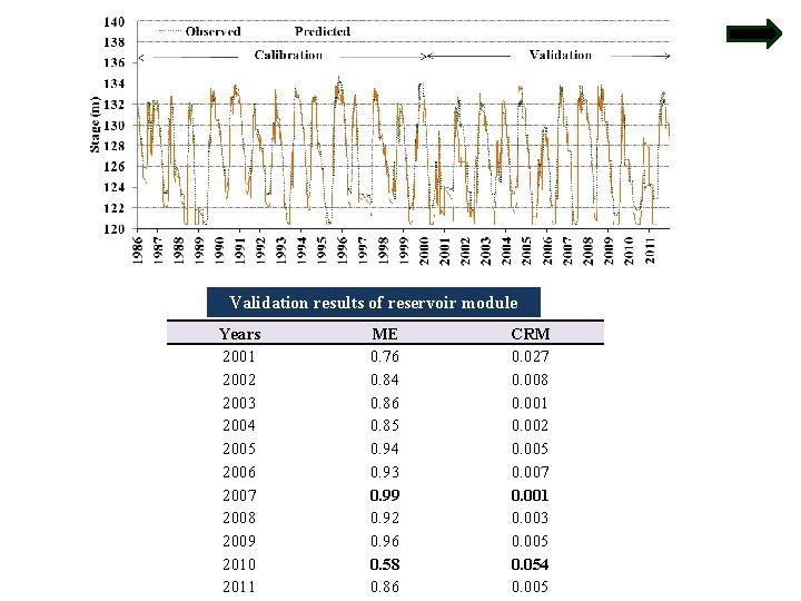
Validation results of reservoir module Years 2001 2002 2003 2004 2005 2006 2007 2008 2009 2010 2011 ME 0. 76 0. 84 0. 86 0. 85 0. 94 0. 93 0. 99 0. 92 0. 96 0. 58 0. 86 CRM 0. 027 0. 008 0. 001 0. 002 0. 005 0. 007 0. 001 0. 003 0. 005 0. 054 0. 005

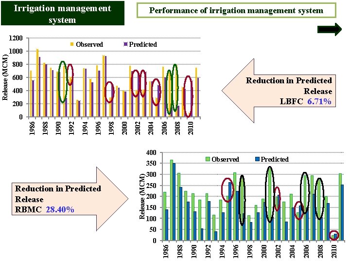
Irrigation management system Observed 1000 Predicted 800 600 Reduction in Predicted Release LBFC 6. 71% 400 2010 2008 2006 2004 400 Observed Predicted 300 250 200 150 100 50 2010 2008 2006 2004 2002 2000 1998 1996 1994 1990 1988 0 1986 Reduction in Predicted Release RBMC 28. 40% Release (MCM) 350 1992 2000 1998 1996 1994 1992 1990 1988 0 1986 Release (MCM) 1200 Performance of irrigation management system

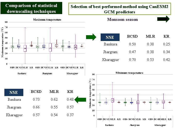
Comparison of statistical downscaling techniques Selection of best performed method using Can. ESM 2 GCM predictors Monsoon season NSE BCSD MLR KR Bankura 0. 73 0. 62 0. 48 Jhargram 0. 66 0. 55 0. 57 Kharagpur 0. 57 0. 54 0. 37 NSE BCSD MLR KR Bankura 0. 50 0. 38 0. 25 Jhargram 0. 47 0. 38 0. 34 Kharagpur 0. 70 0. 53 0. 42

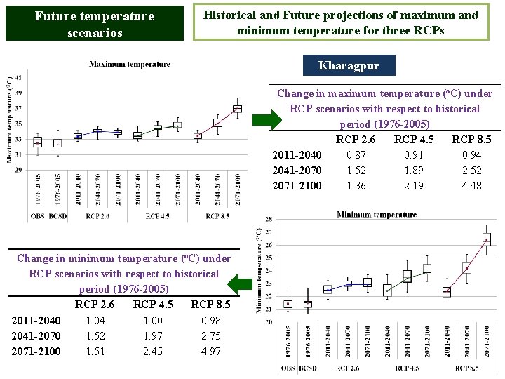
Future temperature scenarios Historical and Future projections of maximum and minimum temperature for three RCPs Kharagpur Change in maximum temperature (o. C) under RCP scenarios with respect to historical period (1976 -2005) RCP 2. 6 RCP 4. 5 RCP 8. 5 2011 -2040 0. 87 0. 91 0. 94 2041 -2070 1. 52 1. 89 2. 52 2071 -2100 1. 36 2. 19 4. 48 Change in minimum temperature (o. C) under RCP scenarios with respect to historical period (1976 -2005) RCP 2. 6 RCP 4. 5 RCP 8. 5 2011 -2040 1. 04 1. 00 0. 98 2041 -2070 1. 52 1. 97 2. 75 2071 -2100 1. 51 2. 45 4. 97

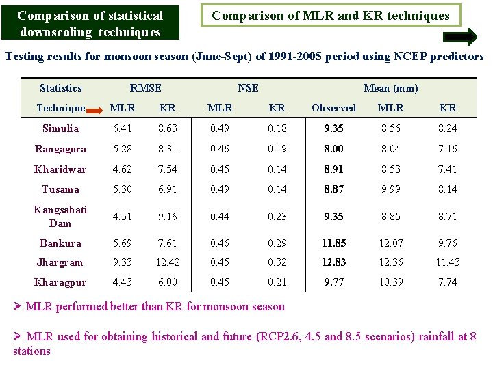
Comparison of statistical downscaling techniques Comparison of MLR and KR techniques Testing results for monsoon season (June-Sept) of 1991 -2005 period using NCEP predictors Statistics RMSE NSE Mean (mm) Technique MLR KR Observed MLR KR Simulia 6. 41 8. 63 0. 49 0. 18 9. 35 8. 56 8. 24 Rangagora 5. 28 8. 31 0. 46 0. 19 8. 00 8. 04 7. 16 Kharidwar 4. 62 7. 54 0. 45 0. 14 8. 91 8. 53 7. 41 Tusama 5. 30 6. 91 0. 49 0. 14 8. 87 9. 99 8. 14 Kangsabati Dam 4. 51 9. 16 0. 44 0. 23 9. 35 8. 85 8. 71 Bankura 5. 69 7. 61 0. 46 0. 29 11. 85 12. 07 9. 76 Jhargram 9. 33 12. 42 0. 45 0. 32 12. 83 12. 36 11. 43 Kharagpur 4. 43 6. 00 0. 45 0. 21 9. 77 10. 39 7. 74 Ø MLR performed better than KR for monsoon season Ø MLR used for obtaining historical and future (RCP 2. 6, 4. 5 and 8. 5 scenarios) rainfall at 8 stations

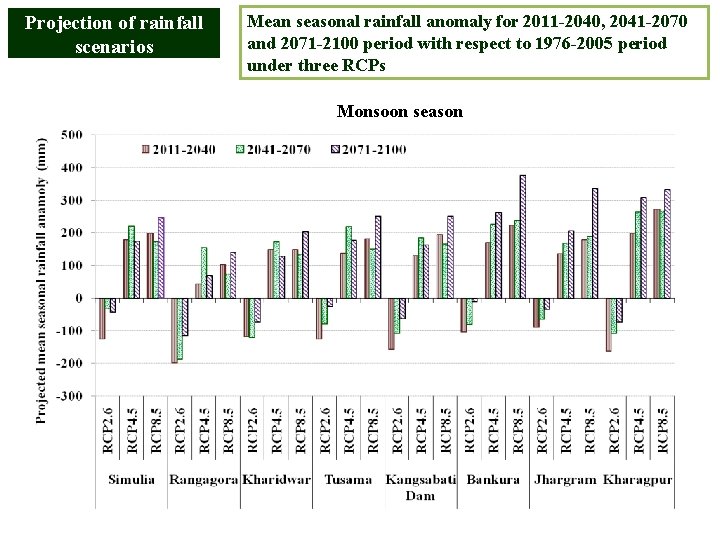
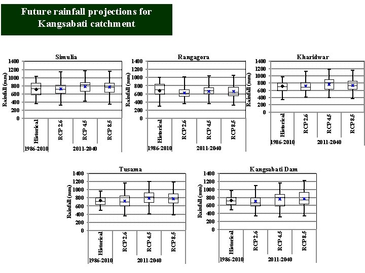
Projection of rainfall scenarios Mean seasonal rainfall anomaly for 2011 -2040, 2041 -2070 and 2071 -2100 period with respect to 1976 -2005 period under three RCPs Monsoon season

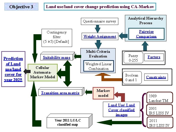
Objective 3 Land use/land cover change prediction using CA-Markov Contingency filter (5 × 5) [Default] Prediction of Land use/land cover for year 2025 Suitability maps Cellular Automata. Markov Model Transition area matrix Questionnaire survey Analytical Hierarchy Process Weight Assignment Pairwise Comparison Multi-Criteria Evaluation Weighted Linear Combination Fuzzy 0 -255 Boolean 0 and 1 Markov model Land Use/ Land Cover classified images Year 2011 LU/LC classified map Factors Constraints 1989 Landsat TM 2001 IRS LISS IV 2011 IRS LISS IV

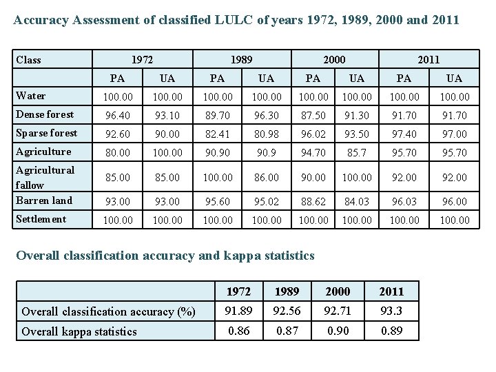
Accuracy Assessment of classified LULC of years 1972, 1989, 2000 and 2011 Class 1972 1989 2000 2011 PA UA Water 100. 00 100. 00 Dense forest 96. 40 93. 10 89. 70 96. 30 87. 50 91. 30 91. 70 Sparse forest 92. 60 90. 00 82. 41 80. 98 96. 02 93. 50 97. 40 97. 00 Agriculture 80. 00 100. 00 90. 9 94. 70 85. 7 95. 70 85. 00 100. 00 86. 00 90. 00 100. 00 92. 00 93. 00 95. 60 95. 02 88. 62 84. 03 96. 00 100. 00 Agricultural fallow Barren land Settlement Overall classification accuracy and kappa statistics 1972 1989 2000 2011 Overall classification accuracy (%) 91. 89 92. 56 92. 71 93. 3 Overall kappa statistics 0. 86 0. 87 0. 90 0. 89

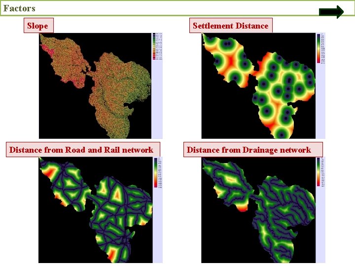
Factors Slope Distance from Road and Rail network Settlement Distance from Drainage network

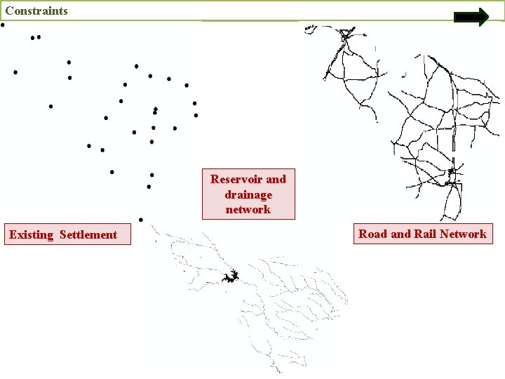
Constraints Reservoir and drainage network Existing Settlement Road and Rail Network

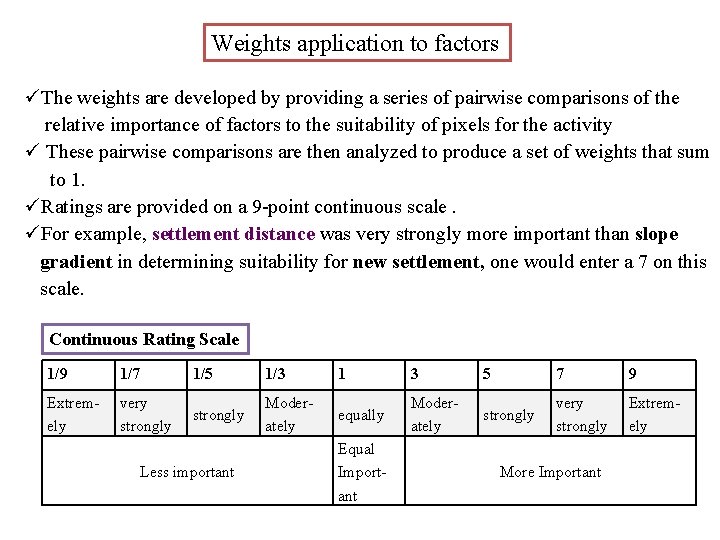
Weights application to factors üThe weights are developed by providing a series of pairwise comparisons of the relative importance of factors to the suitability of pixels for the activity ü These pairwise comparisons are then analyzed to produce a set of weights that sum to 1. üRatings are provided on a 9 -point continuous scale. üFor example, settlement distance was very strongly more important than slope gradient in determining suitability for new settlement, one would enter a 7 on this scale. Continuous Rating Scale 1/9 1/7 1/5 1/3 1 3 5 7 9 Extremely very strongly Moderately equally Moderately strongly very strongly Extremely Less important Equal Important More Important

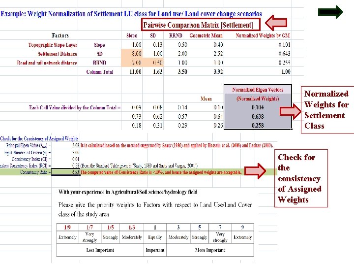
Normalized Weights for Settlement Class Check for the consistency of Assigned Weights

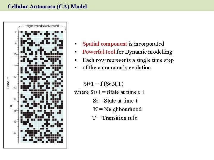
Cellular Automata (CA) Model Spatial component is incorporated Powerful tool for Dynamic modelling § Each row represents a single time step § of the automaton’s evolution. § § St+1 = f (St N, T) where St+1 = State at time t+1 St = State at time t N = Neighbourhood T = Transition rule

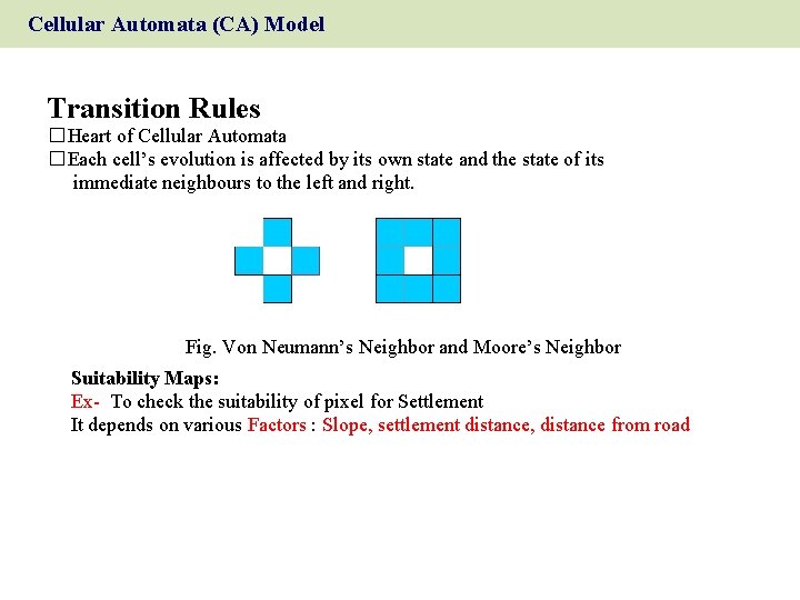
Cellular Automata (CA) Model Transition Rules � Heart of Cellular Automata � Each cell’s evolution is affected by its own state and the state of its immediate neighbours to the left and right. Fig. Von Neumann’s Neighbor and Moore’s Neighbor Suitability Maps: Ex- To check the suitability of pixel for Settlement It depends on various Factors : Slope, settlement distance, distance from road

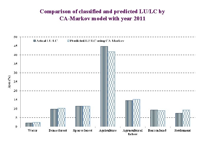
Comparison of classified and predicted LU/LC by CA-Markov model with year 2011

Change in land use/land cover area statistics Actual LU/LC of year 2011 and CA-Markov predicted land use/land cover for year 2025

Irrigation water supply and demand of LBFC command Case II

RCP 8. 5 RCP 2. 6 RCP 4. 5 2011 -2040 RCP 8. 5 Rainfall (mm) 1986 -2010 RCP 4. 5 Historical RCP 2. 6 2011 -2040 Kangsabati Dam Historical Rainfall (mm) RCP 8. 5 RCP 2. 6 RCP 4. 5 2011 -2040 1400 1200 1000 800 600 400 200 0 Kharidwar 1986 -2010 2011 -2040 Tusama 1986 -2010 1400 1200 1000 800 600 400 200 0 RCP 8. 5 RCP 4. 5 RCP 2. 6 Historical 1986 -2010 Historical 1400 1200 1000 800 600 400 200 0 Rangagora 1400 1200 1000 800 600 400 200 0 2011 -2040 Rainfall (mm) 1986 -2010 RCP 8. 5 RCP 4. 5 Rainfall (mm) Simulia RCP 2. 6 1400 1200 1000 800 600 400 200 0 Historical Rainfall (mm) Future rainfall projections for Kangsabati catchment

Future land use scenario for Kangsabati catchment Predicted land use/land cover for year 2025 LU/LC class Area (sq. m ) Water 439. 91 Dense forest 1340. 18 Sparse forest 805. 41 Agriculture 265. 23 Agricultural fallow 358. 95 Barren land 200. 85 Settlement 17. 29

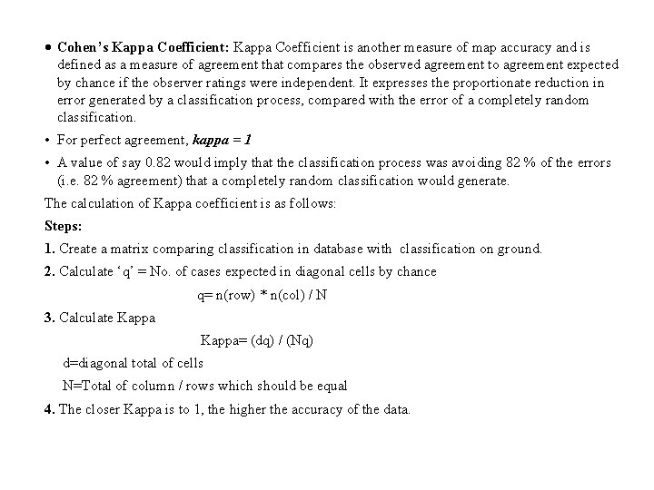
Cohen’s Kappa Coefficient: Kappa Coefficient is another measure of map accuracy and is defined as a measure of agreement that compares the observed agreement to agreement expected by chance if the observer ratings were independent. It expresses the proportionate reduction in error generated by a classification process, compared with the error of a completely random classification. • For perfect agreement, kappa = 1 • A value of say 0. 82 would imply that the classification process was avoiding 82 % of the errors (i. e. 82 % agreement) that a completely random classification would generate. The calculation of Kappa coefficient is as follows: Steps: 1. Create a matrix comparing classification in database with classification on ground. 2. Calculate ‘q’ = No. of cases expected in diagonal cells by chance q= n(row) * n(col) / N 3. Calculate Kappa Kappa= (dq) / (Nq) d=diagonal total of cells N=Total of column / rows which should be equal 4. The closer Kappa is to 1, the higher the accuracy of the data.