ASSESSING RELEASE LIMITS AND MANUFACTURING RISK FROM A

ASSESSING RELEASE LIMITS AND MANUFACTURING RISK FROM A BAYESIAN PERSPECTIVE 1 Areti Manola amanola@its. jnj. com

OUTLINE Introduction � Review Q 1 E Stability Evaluation � Definition of Release Limits Allen, Dukes and Gerger Approach � Mixed Linear Model A Bayesian Approach to Manufacturing Risk Estimation � Bayesian formulation of mixed model � Simulating future lots Posterior predictive distribution Case Studies Summary 2

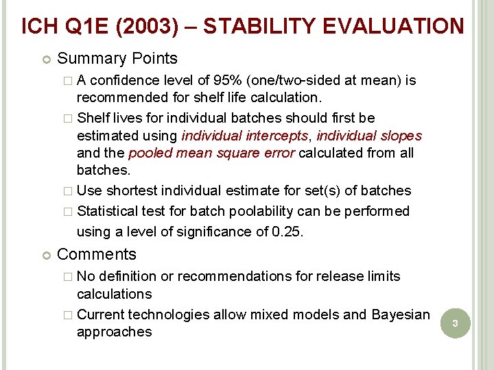
ICH Q 1 E (2003) – STABILITY EVALUATION Summary Points � A confidence level of 95% (one/two-sided at mean) is recommended for shelf life calculation. � Shelf lives for individual batches should first be estimated using individual intercepts, individual slopes and the pooled mean square error calculated from all batches. � Use shortest individual estimate for set(s) of batches � Statistical test for batch poolability can be performed using a level of significance of 0. 25. Comments � No definition or recommendations for release limits calculations � Current technologies allow mixed models and Bayesian approaches 3

DEFINITION OF RELEASE LIMITS Specifications ensure that the identity, strength, quality, and purity of a drug product are maintained throughout its shelf life. Release limits are the bounds of intervals on the true lot mean formed on the basis of given specifications and real time stability data so that a future lot whose measured value at time of manufacture falls within these limits has a high level of assurance that its mean will remain within specifications throughout shelf life. 4

RELEASE LIMITS Internally derived and are the responsibility of the manufacturer, lot acceptance limits Apply only at time of lot release Account for changes over time and uncertainties due to process variability Intended to provide a high level of assurance that a lot falling within release limits will conform to quality requirements over the shelf life of the product Important to the customer ØGiven Release Limits and Specifications how can we assess manufacturing risk? 5

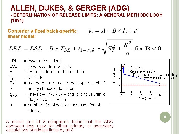
ALLEN, DUKES, & GERGER (ADG) - DETERMINATION OF RELEASE LIMITS: A GENERAL METHODOLOGY (1991) Consider a fixed batch-specific linear model: Percent of Label LRL = lower release limit LSL = lower specification limit B = average slope for degradation TSL = shelf life ST = standard error of average slope shelf life S = assay standard deviation t 1 -a, k = one-sided (1 -a)%-ile critical t value with k degrees of freedom n = number of replicate assays used for lot release 105% 100% 95% Release Assay + Regression Loss Uncertainty Regression Loss 90% 85% 0 6 12 18 Time (Months) 24 6 A recent poll of 8 companies found that the ADG approach was used for either primary or secondary calculations of release limits by all 8

OTHER APPROACHES Shao and Chow (1991) Constructing Release Targets for Drug Products: a Bayesian Decision Theory Approach Various choices of release limits are viewed as part of an action space; an action is chosen so as to minimize the cost through an appropriately chosen loss function Greg C. G. Wei (1998) Simple Methods for Determination of the Release Limits for Drug Products “Conditional “ release limits (control the chance of failure for a given lot - similar to Allen’s method) and “Unconditional” release limits (control the chance of failure for all future lots); expected loss function approach that minimizes cost due to lot failures at T 0 & TSL Murphy and Hofer (2002) Establishing Shelf life, Expiry Limits and Release Limits Conditions shelf life on control limits at time of release 7

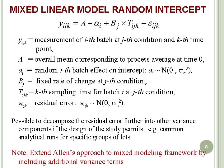
MIXED LINEAR MODEL RANDOM INTERCEPT yijk = measurement of i-th batch at j-th condition and k-th time point, A = overall mean corresponding to process average at time 0, αi = random i-th batch effect on intercept: αi ~ N(0 , α 2), Bj = fixed rate of change at j-th condition, Tijk = k-th sampling time for batch i at j-th condition, ijk = residual error: ijk ~ N(0, ε 2). Possible to decompose the residual error further into other variance components if the design of the study permits, e. g. common analytical runs for specific groups of lots 8 Note: Extend Allen’s approach to mixed modeling framework by including additional variance terms

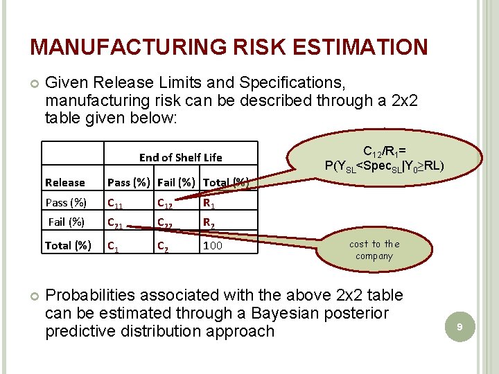
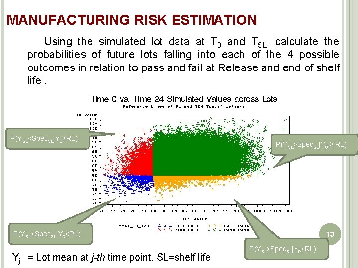
MANUFACTURING RISK ESTIMATION Given Release Limits and Specifications, manufacturing risk can be described through a 2 x 2 table given below: End of Shelf Life Release Pass (%) Fail (%) Total (%) Pass (%) C 11 C 12 R 1 Fail (%) C 21 C 22 R 2 Total (%) C 1 C 2 100 C 12/R 1= P(YSL<Spec. SL|Y 0≥RL) cost to the company Probabilities associated with the above 2 x 2 table can be estimated through a Bayesian posterior predictive distribution approach 9

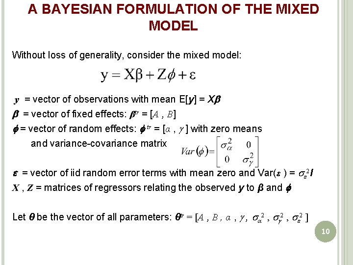
A BAYESIAN FORMULATION OF THE MIXED MODEL Without loss of generality, consider the mixed model: y = vector of observations with mean E[y] = X = vector of fixed effects: βtr = [A , B] f = vector of random effects: f tr = [α , ] with zero means and variance-covariance matrix = vector of iid random error terms with mean zero and Var(ε ) = 2 I X , Z = matrices of regressors relating the observed y to β and f Let θ be the vector of all parameters: θtr = [A , B , α , , 2 ] 10

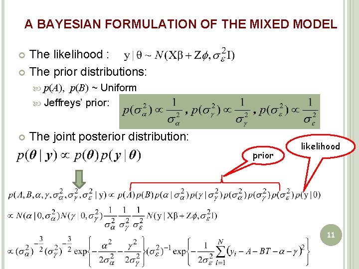
A BAYESIAN FORMULATION OF THE MIXED MODEL The likelihood : The prior distributions: p(A), p(B) ~ Uniform Jeffreys’ prior: The joint posterior distribution: prior likelihood 11

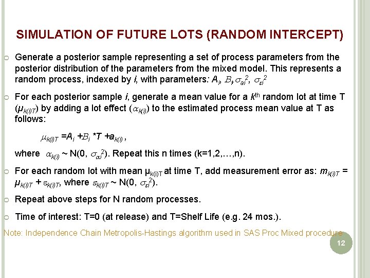
SIMULATION OF FUTURE LOTS (RANDOM INTERCEPT) Generate a posterior sample representing a set of process parameters from the posterior distribution of the parameters from the mixed model. This represents a random process, indexed by i, with parameters: Ai, Bi, ai 2, i 2 For each posterior sample i, generate a mean value for a kth random lot at time T (µk(i)T) by adding a lot effect ( k(i)) to the estimated process mean value at T as follows: mk(i)T =Ai +Bi *T +ak(i) , where k(i) ~ N(0, i 2). Repeat this n times (k=1, 2, …, n). For each random lot with mean µk(i)T at time T, add measurement error as: mk(i)T = µk(i)T + k(i)T, where k(i)T ~ N(0, i 2). Repeat above steps for N random processes. Time of interest: T=0 (at release) and T=Shelf Life (e. g. 24 mos. ). Note: Independence Chain Metropolis-Hastings algorithm used in SAS Proc Mixed procedure 12

MANUFACTURING RISK ESTIMATION Using the simulated lot data at T 0 and TSL, calculate the probabilities of future lots falling into each of the 4 possible outcomes in relation to pass and fail at Release and end of shelf life. P(YSL<Spec. SL|Y 0≥RL) P(YSL>Spec. SL|Y 0 ≥ RL) P(YSL<Spec. SL|Y 0<RL) Yj = Lot mean at j-th time point, SL=shelf life 13 P(YSL>Spec. SL|Y 0<RL)

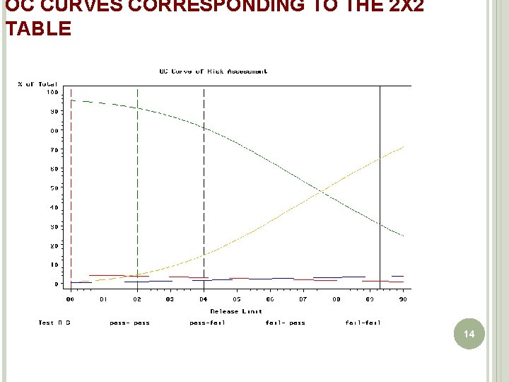
OC CURVES CORRESPONDING TO THE 2 X 2 TABLE 14

CASE STUDIES 15

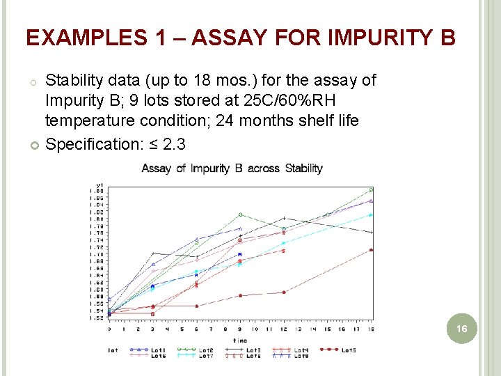
EXAMPLES 1 – ASSAY FOR IMPURITY B Stability data (up to 18 mos. ) for the assay of Impurity B; 9 lots stored at 25 C/60%RH temperature condition; 24 months shelf life Specification: ≤ 2. 3 o 16

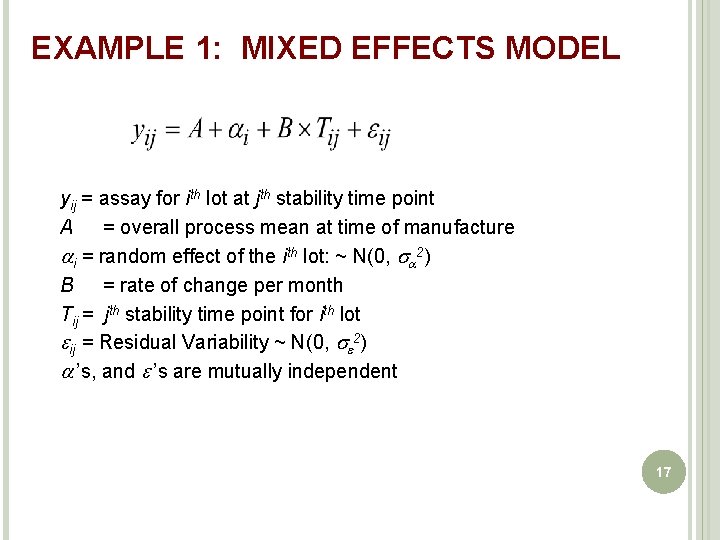
EXAMPLE 1: MIXED EFFECTS MODEL yij = assay for ith lot at jth stability time point A = overall process mean at time of manufacture i = random effect of the ith lot: ~ N(0, 2) B = rate of change per month Tij = jth stability time point for ith lot ij = Residual Variability ~ N(0, 2) ’s, and ’s are mutually independent 17 17

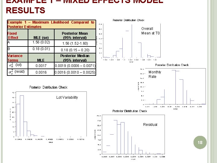
EXAMPLE 1 – MIXED EFFECTS MODEL RESULTS Example 1 – Maximum Likelihood Compared to Posterior Estimates Fixed Effect A Posterior Mean (95% interval) MLE (se) 1. 56 (0. 02) B 0. 18 (0. 01) 0. 18 (0. 15 – 0. 20) Overall Mean at T 0 1. 56 (1. 52 -1. 60) Variance Terms (lot) MLE Posterior Median (95% interval) 0. 0017 0. 0019 (0. 0006 – 0. 0071) (resid) 0. 0016 (0. 0010 – 0. 0025) Monthly Rate Lot Variability Residual 18

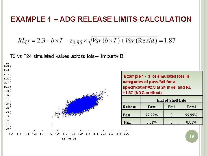
EXAMPLE 1 – ADG RELEASE LIMITS CALCULATION Example 1 - % of simulated lots in categories of pass/fail for a specification=2. 3 at 24 mos. and RL =1. 87 (ADG method) Release End of Shelf Life Pass Fail Total Pass 99. 99% 0 99. 99% Fail 0. 01% 0 0. 01% 19

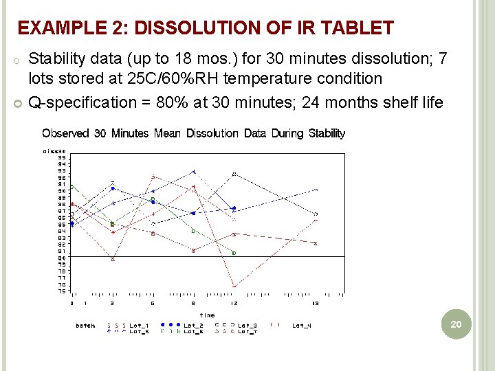
EXAMPLE 2: DISSOLUTION OF IR TABLET Stability data (up to 18 mos. ) for 30 minutes dissolution; 7 lots stored at 25 C/60%RH temperature condition Q-specification = 80% at 30 minutes; 24 months shelf life o 20

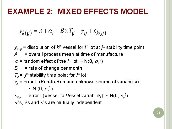
EXAMPLE 2: MIXED EFFECTS MODEL yk(ij) = dissolution of kth vessel for ith lot at jth stability time point A = overall process mean at time of manufacture i = random effect of the ith lot: ~ N(0, 2) B = rate of change per month Tij = jth stability time point for ith lot ij = error II (Run-to-Run and unknown source of variability): ~ N (0, 2 ) k(ij) = error I (Vessel-to-Vessel variability): ~ N(0, 2) ’s, ’s and ’s are mutually independent 21 21

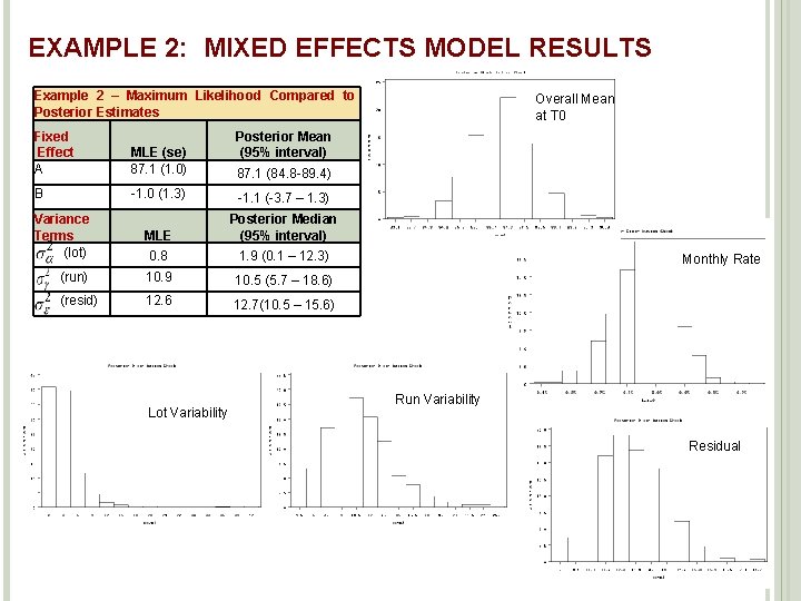
EXAMPLE 2: MIXED EFFECTS MODEL RESULTS Example 2 – Maximum Likelihood Compared to Posterior Estimates Fixed Effect A MLE (se) 87. 1 (1. 0) B -1. 0 (1. 3) -1. 1 (-3. 7 – 1. 3) Variance Terms (lot) MLE Posterior Median (95% interval) 0. 8 1. 9 (0. 1 – 12. 3) (run) 10. 9 10. 5 (5. 7 – 18. 6) (resid) 12. 6 12. 7(10. 5 – 15. 6) Lot Variability Overall Mean at T 0 Posterior Mean (95% interval) 87. 1 (84. 8 -89. 4) Monthly Rate Run Variability Residual 22

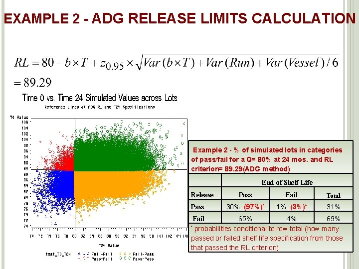
EXAMPLE 2 - ADG RELEASE LIMITS CALCULATION Example 2 - % of simulated lots in categories of pass/fail for a Q= 80% at 24 mos. and RL criterion= 89. 29(ADG method) Release Pass End of Shelf Life Pass Fail Total 30% (97%)* 1% (3%)* 31% Fail 65% 4% 69% * probabilities conditional to row total (how many 23 passed or failed shelf life specification from those that passed the RL criterion)

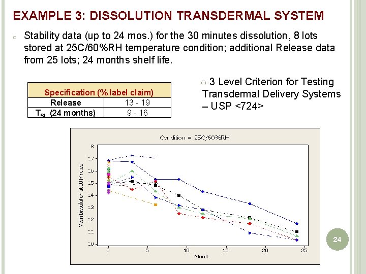
EXAMPLE 3: DISSOLUTION TRANSDERMAL SYSTEM o Stability data (up to 24 mos. ) for the 30 minutes dissolution, 8 lots stored at 25 C/60%RH temperature condition; additional Release data from 25 lots; 24 months shelf life. Specification (% label claim) Release 13 - 19 TSL (24 months) 9 - 16 o 3 Level Criterion for Testing Transdermal Delivery Systems – USP <724> 24

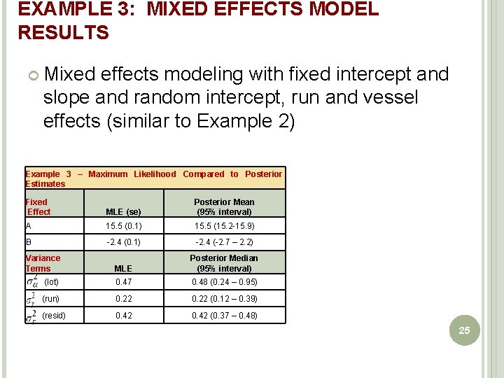
EXAMPLE 3: MIXED EFFECTS MODEL RESULTS Mixed effects modeling with fixed intercept and slope and random intercept, run and vessel effects (similar to Example 2) Example 3 – Maximum Likelihood Compared to Posterior Estimates Fixed Effect MLE (se) Posterior Mean (95% interval) A 15. 5 (0. 1) 15. 5 (15. 2 -15. 9) B -2. 4 (0. 1) -2. 4 (-2. 7 – 2. 2) Variance Terms MLE Posterior Median (95% interval) (lot) 0. 47 0. 48 (0. 24 – 0. 95) (run) 0. 22 (0. 12 – 0. 39) (resid) 0. 42 (0. 37 – 0. 48) 25

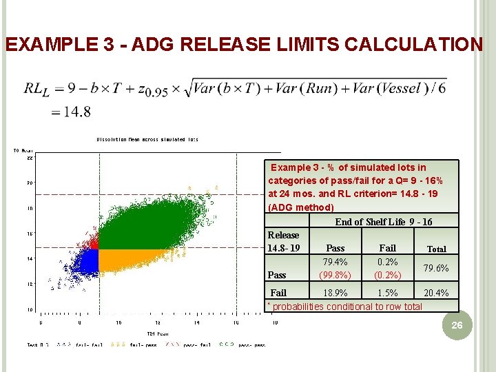
EXAMPLE 3 - ADG RELEASE LIMITS CALCULATION Example 3 - % of simulated lots in categories of pass/fail for a Q= 9 - 16% at 24 mos. and RL criterion= 14. 8 - 19 (ADG method) End of Shelf Life 9 - 16 Release 14. 8 - 19 Pass Fail Total 79. 4% 0. 2% 79. 6% Pass (99. 8%) (0. 2%) Fail 18. 9% 1. 5% 20. 4% * probabilities conditional to row total 26

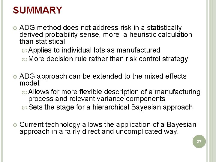
SUMMARY ADG method does not address risk in a statistically derived probability sense, more a heuristic calculation than statistical. Applies to individual lots as manufactured More decision rule rather than risk control strategy ADG approach can be extended to the mixed effects model. Allows for more flexible description of a manufacturing process and relevant variance components Sets the stage for a hierarchical Bayesian approach Current technology allows the application of a Bayesian approach in a fairly direct and uncomplicated way. 27

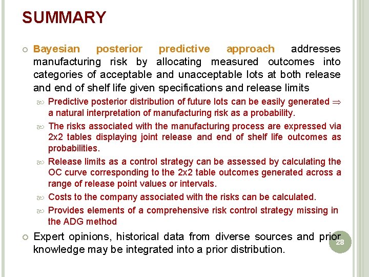
SUMMARY Bayesian posterior predictive approach addresses manufacturing risk by allocating measured outcomes into categories of acceptable and unacceptable lots at both release and end of shelf life given specifications and release limits Predictive posterior distribution of future lots can be easily generated a natural interpretation of manufacturing risk as a probability. The risks associated with the manufacturing process are expressed via 2 x 2 tables displaying joint release and end of shelf life outcomes as probabilities. Release limits as a control strategy can be assessed by calculating the OC curve corresponding to the 2 x 2 table outcomes generated across a range of release point values or intervals. Costs to the company associated with the risks can be calculated. Provides elements of a comprehensive risk control strategy missing in the ADG method Expert opinions, historical data from diverse sources and prior 28 knowledge may be integrated into a prior distribution.

REFERENCES Allen, Dukes, & Gerger (1991). Determination of Release Limits: A General Methodology. Pharmaceutical Research, Vol. 8, No. 9, pp. 1210 -1213. Shao and Chow (1991). Constructing Release Targets for Drug Products: a Bayesian Decision Theory Approach. JRSS, Series C (Applied Statistics) 1991, 40, No. 3, pp. 381 -390. Greg C. G. Wei (1998). Simple Methods for Determination of the Release Limits for Drug Products. Journal of Biopharmaceutical Statistics, 1998, 8(1), 103 -114. Murphy and Hofer (2002). Establishing Shelf life, Expiry Limits and Release Limits. Drug Information Journal, 2002, vol. 36, pp. 769 -781. Andrew Gelman, John B. Carlin, Hal S. Stern and Donald B. Rubin (2004). Bayesian Data Analysis. 2 nd ed. Chapman & Hall/CRC. 29