ASR Feature Extraction Training Search and Evaluation Julia

ASR Feature Extraction, Training, Search and Evaluation Julia Hirschberg COMS 4706

Noisy Channel Model likelihood 11/1/2020 Speech and Language Processing Jurafsky and Martin prior 2

Speech Recognition Architecture 11/1/2020 3

ASR Components • ASR Architecture – Feature Extraction procedure – Lexicon/Pronunciation Model – Acoustic Model – Language Model (Ngrams) – Decoder – Evaluation 11/1/2020 4

ASR Components • ASR Architecture – Feature Extraction procedure – Lexicon/Pronunciation Model – Acoustic Model – Language Model (Ngrams) – Decoding – Evaluation 11/1/2020 5

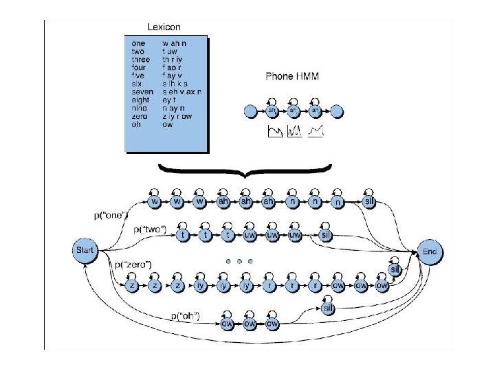
ASR Process • Choose a method to extract acoustic information • Create an Acoustic Model (AM) to compute P(O|W) – Build an HMM for each word in lexicon – Expand word HMMs to phone HMMs – Build a ‘whole sentence’ HMM for each sentence in the training data (embedded training) – Compute transition probabilities (A) and observation likelihoods (B) • Create a Language Model (LM) to compute P(W)

– Compute ngram log probabilities from very large text corpus and store in lookup table • Choose a Decoding strategy – Use AM and LM to recognize new data • Choose an evaluation strategy to measure success

Today • • Feature extraction Embedded training using Baum-Welch Decoding using Viterbi Evaluation methods

Feature Extraction • Digitize the signal (A/D) – Sample at : 16 KHz (wideband) or 8 KHz (telephone) – Convert real amplitude values to integer • Boost energy in higher frequencies (pre-emphasis) – Balancing spectral tilt improves phone recognition • Divide signal into overlapping frames (windowing) – Capture stationary parts of spectrum – Hamming windowing avoids discontinuities between windows • Perform Discrete Fourier Transform (DFT) to extract spectral data (energy) for each frequency band

• Compute Mel Frequency Cepstral Coefficients (MFCCs) to convert DFT output to the mel scale – Log scale above 1000 Hz to mimic human hearing – Compute log of mel spectrum to reduce sensitivity to power variation • Compute cepstrum (spectrum of log of spectrum) to separate source (from vocal folds) from filter (vocal tract) to better identify phones – Cepstral coefficients represent f 0 and harmonics information, so we can use only harmonics – Include delta and delta-delta cepstrum to capture change • Compute energy

Pre-emphasis • Before and after pre-emphasis – Spectral slice from the vowel [aa] 11/1/2020 Speech and Language Processing Jurafsky and Martin 11

MFCC process: windowing 11/1/2020 Speech and Language Processing Jurafsky and Martin 12

MFCC process: windowing 11/1/2020 Speech and Language Processing Jurafsky and Martin 13

Discrete Fourier Transform computing a spectrum • A 25 ms Hamming-windowed signal from [iy] – And its spectrum as computed by DFT (plus other smoothing) 11/1/2020 Speech and Language Processing Jurafsky and Martin 14

Mel-scale • Human hearing is not equally sensitive to all frequency bands • Less sensitive at higher frequencies, roughly > 1000 Hz • I. e. human perception of frequency is non-linear: 11/1/2020 Speech and Language Processing Jurafsky and Martin 15

Cepstrum: Spectrum of the log of the Spectrum Log spectrum Spectrum of log spectrum 11/1/2020 Speech and Language Processing Jurafsky and Martin 16

MFCC: Mel-Frequency Cepstral Coefficients 11/1/2020 Speech and Language Processing Jurafsky and Martin 17

Typical MFCC features Window size: 25 ms Window shift: 10 ms Pre-emphasis coefficient: 0. 97 MFCC: – 12 MFCC (mel frequency cepstral coefficients) – 1 energy feature – 12 delta MFCC features – 12 double-delta MFCC features – 1 delta energy feature – 1 double-delta energy feature • Total 39 -dimensional features • • 11/1/2020 18

Speech Recognition Architecture 11/1/2020 19

Embedded Training • Given a training corpus, with sentences segmented and orthographically transcribed and a pronouncing lexicon • Build HMMs for each sentence • Initialize transition probabilities (A) and observation likelihoods (B) to neutral weights • Re-estimate A and B by iterating Baum-Welch or Viterbi algorithm over corpus until convergence

Baum-Welch (Forward-Backward) Algorithm • Goal: Learn HMM parameters: transition probabilities A between the states and emission probabilities B for each state – How likely are we to transition from state i to state j? – How likely are we to be in state j if we observation o? • We’d like to just count the # of times a transition from i to j occurs and normalize by the total # of transitions from i • But -- for a given observation sequence, if we are now in state j, we have no record of how we got here

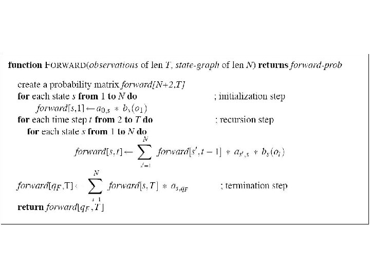
• BW intuition: – Estimate transition counts iteratively – Get estimates by computing the forward probability for an observation and dividing the probability mass among all the paths that might have gotten us there • Forward probability: the likelihood of being in a state j in an HMM after seeing t observations • Backward probability: the probability of seeing the observations from t+1 to the end, given that we are at state j at time t in an HMM • Together these estimate a path from start to end going through j

BW: Forward Algorithm • Dynamic programming algorithm – Fills cells in trellis recursively – Each cell αi(j) represents the probability of being in state qj of the HMM after seeing the first t observations – Calculated by multiplying, for all previous paths • αt-1(i): the previous forward path probability • αij : the transition probability from previous state qi to current state qj • bj(ot): the observation likelihood of ot at state qj – Add them up – O(N 2 T) time, where T is the length of the observation sequence

Forward Algorithm: Summing over all possible sequences of states • A simple example: “five” – f ay ay v v – f f ay ay v v v – f f ay ay ay ay ay v – f f ay v v v v

First 3 Time Steps of Forward Lattice for “five”

The Forward Trellis for “five”

BW: The Backward Probability • Initialization • Recursion • Termination

Computing βt(i)

Finishing Baum-Welch • So how do we estimate how likely a transition is from i to j given an input O and an HMM λ? • We need to compute âij=expected transitions from i to j/expected number of transitions from i • The Forward (α) and Backward (β) probabilities get us close to estimating âij if we think of the numerator as a joint probability ξt (i, j)=P(qt=i, qt+1=j|O, λ) – Now, we include O in the joint probability -~ξt(i, j)=P(qt=i, qt+1=j, O| λ) – Next, we define the probabilities that go into computing ~ξt (i, j) in terms of α and β

Figure 6. 14

• Now we have ~ξt(i, j)=αt(i)*aij*bj(ot+1)*βt+1(j) • We divide by the probability of O given λ, which turns out to be just the Forward (or Backward) probability of the whole utterance • So, ξt(i, j)=αt(i)*aij*bj(ot+1)*βt+1(j) / αT(q. F) is our estimate of the transitions from i to j given O and λ at time t • We must sum over all times t in O to get the expected number of transitions from i to j at any point when O is being processed • We also need to compute our denominator – what are the total # of transitions from state i – but we can use the same equation

• So we have • We must also compute the observation probabilities b’j(vk) = How often are we in state j when we observation o/how often are we in j at all, given O and λ – We use ϒt(j), the probability of being in state j at time t, which we can compute using α and β • Now, given an initial estimation of the A and B probabilities, we do the following: – E-step: estimate ξt (i, j) and ϒt(j) – M-step: use these to compute âij and b’j(vk) and update the A and B tables of our HMM λ

So, How do we do Recognition? • Given: A wave file (no transcription) • Goal: output a string of words • What we have: – A feature extraction module that extracts MFCC vectors for each 10 ms window of the input – An acoustic model with trained transition probabilities and observation likelihoods – A language model with trained ngram probabilities • How do we put this together? 11/1/2020 34

Why is ASR decoding hard? • Decoder must segment the utterance and identify the words at the same time

Decoding • In principle: • In practice: – We need to give the acoustic model more weight and correct for the LM’s tendency to prefer longer words – So….

Decoding: Finding the Best Sequence of (Hidden) Phones • How do we find the most likely sequence of (hidden) states that generated the acoustic observations? – For each possible (hidden) state sequence, we could run the Forward Algorithm and compute the likelihood of the observation sequence to find the state sequence with the maximum observation likelihood – But there an exponentially large number of state sequences • So we use a more efficient algorithm that looks a lot like the Forward Algorithm -- the Viterbi Algorithm

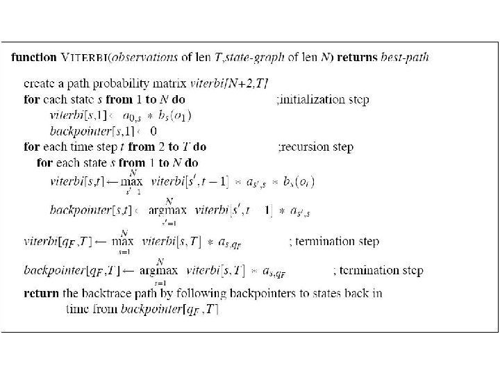
The Viterbi Algorithm • Dynamic Programming Algorithm – Each cell in trellis represents the probability that the HMM is in state qi after seeing t observations and passing thru the most probable state sequence in the HMM – Cell vt(j) computed by multiplying • the Viterbi path probability vt-1(i) from the most probable previous state qi • the transition probability from that state qi • the state observation likelihood of the input ot in qj

• Like the Forward Algorithm except – It takes the max over the previous path probabilities rather than the sum – It maintains backpointers so the best path can be backtraced to the start state at the end of the computation – Probabilities are different, since they come from a single path

Viterbi Trellis for “five”

Viterbi Trellis for “five”

Decoding Word Sequences from HMM States • We have a path thru HMM states, so how do we figure out the words? • Augment transition matrix (A) with interword probability of transitioning from end of w 1 to beginning of w 2 • Use ngram LM priors (P(W)) to model transitions between words in HMM • Once Viterbi trellis computed – Start from most probable state at tn – Follow backtrace ptrs to get most probable string of states: most probable string of words

Search Space with Bigrams

Viterbi trellis

Viterbi Backtrace

Pruning and Beam Search • Viterbi better than Forward Algorithm but still slow – what can we do? • Prune low probability paths at each time step • Beam Search: – At each time t, compute probability of best state/path D – Prune any state worse than D by a threshold (beam width) θ – Improves performance significantly

Evaluation • How do we evaluate the word string output by a speech recognizer?

Word Error Rate • Word Error Rate = 100 (Insertions+Substitutions + Deletions) ---------------Total Word in Correct Transcript Aligment example: REF: portable **** PHONE UPSTAIRS last night so HYP: portable FORM OF STORES last night so Eval I S S WER = 100 (1+2+0)/6 = 50%

NIST sctk-1. 3 scoring softare: Computing WER with sclite • http: //www. nist. gov/speech/tools/ • Sclite aligns a hypothesized text (HYP) (from the recognizer) with a correct or reference text (REF) (human transcribed) id: (2347 -b-013) Scores: (#C #S #D #I) 9 3 1 2 REF: was an engineer SO I i was always with **** MEN UM and they HYP: was an engineer ** AND i was always with THEM THEY ALL THAT and they Eval: D S I I S S

Sclite output for error analysis CONFUSION PAIRS Total (972) With >= 1 occurances (972) 1: 2: 3: 4: 5: 6: 7: 8: 9: 10: 11: 12: 13: 14: 15: 16: 6 -> (%hesitation) ==> on 6 -> the ==> that 5 -> but ==> that 4 -> a ==> the 4 -> four ==> for 4 -> in ==> and 4 -> there ==> that 3 -> (%hesitation) ==> and 3 -> (%hesitation) ==> the 3 -> (a-) ==> i 3 -> and ==> in 3 -> are ==> there 3 -> as ==> is 3 -> have ==> that 3 -> is ==> this

Sclite output for error analysis 18: 19: 20: 21: 22: 23: 24: 25: 26: 27: 28: 29: 30: 31: 32: 33: 34: 17: 3 3 2 2 2 2 3 -> -> -> -> -> it ==> that mouse ==> most was ==> is was ==> this you ==> we (%hesitation) ==> it (%hesitation) ==> that (%hesitation) ==> to (%hesitation) ==> yeah a ==> all a ==> know a ==> you along ==> well and ==> it and ==> we and ==> you are ==> i are ==> were

Better Metrics than WER? • WER has been useful • But should we be more concerned with meaning (“semantic error rate”)? – Good idea, but hard to agree on domain concepts – Has been applied in dialogue systems, where desired semantic output may be more clear – Just like WER but defined in terms of concepts, not words

Summary: ASR Architecture • ASR Noisy Channel architecture 1) Feature Extraction: 39 “MFCC” features 2) Acoustic Model: Gaussians for computing p(o|w) 3) Lexicon/Pronunciation Model • HMM: what CD phones can follow each other for computing p(o|w) 4) Language Model for computing p(w) • Probability of N-grams in context, e. g. p(wi|wi-1) 5) Decoder • Viterbi algorithm: dynamic programming for combining all these to get best word sequence from speech 6) Evaluation • Metric for determining success, improvement

Next Class • Spoken Dialogue Systems • Proj 2 due 4/11 at 11: 59 pm