ASL 761 Earth System Modeling Sandeep Sahany Room

ASL 761: Earth System Modeling Sandeep Sahany Room 413, Block VI, Centre for Atmospheric Sciences, IIT Delhi E-mail: ssahany@cas. iitd. ac. in Course Material: http: //web. iitd. ac. in/~ssahany/ASL 761/

Hierarchical Numerical Modeling

Single column model • • • It is a one-dimensional prognostic model Essentially a single column of a full GCM These are building blocks of a GCM/RCM that interact with each other via the large-scale dynamics Simulates the time evolution of a single atmospheric column While the physics remains the same, the dynamics gets replaced by a simpler version

Single column model • Initial Conditions: Ps, T profile, q profile, u profile, v profile, surface temperature and soil moisture • Boundary Conditions: Solar constant, surface characteristics (elevation, albedo, roughness, vegetation type, etc. ), profile of large-scale advection of u, v, T and q, and profile of pressure gradient force

Governing Laws and Equations

ECMWF Tutorial

ECMWF Tutorial

ECMWF Tutorial

Single column model • Parameterization: A way of representing the impact of sub-grid processes on the resolved model state • Say for example we need to test a new deep convective parameterization scheme that has been developed for a GCM: How to check if this parameterization is better than the previous version?

Single column model • Use 2 versions of the SCM – one with the previous physics, and the other with “new” physics • Force the model with initial and boundary conditions obtained from observations and integrate the 2 model versions • Validate against column observations • If the error is less the new version is better than the previous, else vice-versa • What are the advantages and disadvantages of an SCM?

Single column model Primary advantages are: ü reduced computational cost (can be run even on a PC) ü quick first-order validation without caring too much about details ü Allows to compare physics packages regardless of dynamics

Single column model Primary disadvantages are: ü Errors that arise due to feedbacks with the large-scale circulation are unknown ü Strong dependence on the quality and setting of the large-scale forcing

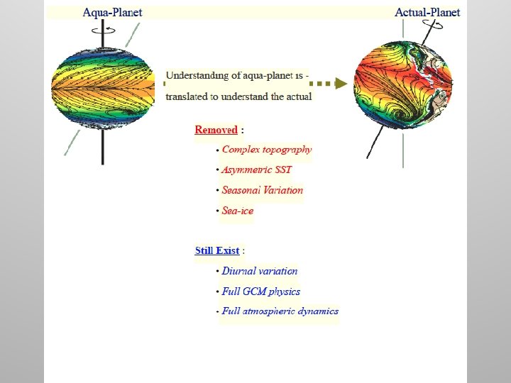
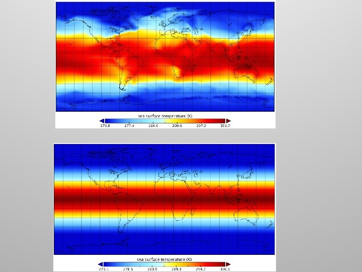
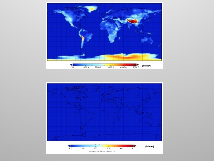
ASL 761 Hierarchical Numerical Modeling - Aquaplanets

An aquaplanet simulation from the Nonhydrostatic Icosahedral Atmospheric Model (NICAM)

Objective • A test-bed for testing interactions of dynamics and physical parameterizations in atmospheric GCMs • Provides a way of intercomparison of different climate models but with simpler forcing, and boundary conditions

Notes • Fills in the gap between an AGCM and an SCM • The feedback between the physics and large-scale dynamics is retained • Very idealized SST distributions • “Correct” solution is not known for these tests • Although theoretical constraints exist

Experimental Set-up • Initialized from the atmospheric state produced from a full AGCM • An 18 -month integration is performed • Adjustment to a change in the underlying SST generally occurs within the first 6 months of model integration • Final 12 -month period is used for analysis • Differences in simulations (between a longerperiod and 12 -month period) small compared to differences in the individual experiments

Deep Convection - Stage 1 ü In an unstable environment, once air is lifted to the level of free convection (LFC), it will continue to rise as long as it is warmer (in terms of Tv) than the air around it. ü The uppermost level is the Equilibrium Level (EL).

Deep Convection - Stage 2 ü Eventually, the parcel reaches an EL at which its virtual temperature equals that of the surrounding environment. ü As the parcel carries a certain amount of upward momentum, some additional ascent will occur beyond the EL. ü This additional rise forms overshooting top above the anvil. an ü Finally, the parcels become now cooler than their surrounding environment, and so they sink back towards the EL. ü Subsequently, the parcels may oscillate vertically about the EL, dampening with time.

Cont. . . ü As the process repeats, air parcels accumulate at this level and spread laterally, creating the cloud anvil. ü While all this is going on, moisture is condensing in the rising updraft air. The weight of the condensed moisture will eventually be too much for the updraft to hold aloft. ü As a result, precipitation will begin to fall back down through the updraft.

Deep Convection - Stage 3 ü Falling precipitation drags air downward and at the initial stages this is the most significant contributor to the strength of a downdraft. ü Evaporation of rain into: (i) the drier air entrained by the downdraft and (ii) as it falls below the cloud base. ü Both of these processes make the downdraft colder than the surrounding air, further enhancing its downward acceleration.

Deep Convection - Stage 4 ü When the downdraft reaches the surface it spreads out, forming the cold pool. ü The downdraft and spreading cold pool represent the final stages in the life cycle of the cell. ü At this point, the buoyancy has all become negative.

Case Study – Convective Downdraft Sensitivity • Zhang-Mac. Farlane (ZM) deep convective parameterization is used in the NCAR CESM model • Simplified form of the Initial Downdraft Mass Flux, Md = α * Mu • ZM Assumption: Convective downdraft starts at or below the bottom of the updraft detrainment layer • ZM Assumption: Convective downdraft is maintained in a saturated state by evaporation of deep convective precipitation produced at a given level • ZM Assumption: Exist only if there is precipitation production in the updraft

Experimental Set-up • An 18 -month integration is performed • First 6 months discarded as spin-up • Final 12 -month period is used for analysis

Case Study – Convective Downdrafts Sensitivity Deep Convective Rainfall Area averaged, time mean values versus alpha for the region (0 E to 360 E and 7 S to 7 N). The error bars show the respective standard deviation about the mean values. Sahany and Nanjundiah, 2008

Case Study – Convective Downdrafts Sensitivity DRF Production Area averaged, time mean values for the region (0 E to 360 E and 7 S to 7 N) Sahany and Nanjundiah, 2008

Case Study – Convective Downdrafts Sensitivity Precipitation Evaporation into Downdrafts Area averaged, time mean values for the region (0 E to 360 E and 7 S to 7 N) Sahany and Nanjundiah, 2008

Case Study – Convective Downdrafts Sensitivity Net Production of Deep Convective Precipitation Area averaged, time mean values for the region (0 E to 360 E and 7 S to 7 N) Sahany and Nanjundiah, 2008

Case Study – Convective Downdrafts Sensitivity Deep Convective Rainfall Area averaged, time mean values versus alpha for the region (0 E to 360 E and 7 S to 7 N). The error bars show the respective standard deviation about the mean values. Sahany and Nanjundiah, 2008

AGCM • An AGCM needs prescribed SSTs as the lower boundary forcing • If one wants to predict the SSTs, there are 2 options: ü AGCM + slab ocean model ü Coupled Model (fully functional ocean model)

AGCM + Slab Ocean • The mixed layer depth of the ocean is assumed to be constant (can vary in space, not time) • For the slab ocean an internal heat source ‘Q’ (also called Q flux) is prescribed such that it represents the climatological conditions • The Q flux consists of seasonal deep water exchange and horizontal heat transport • Allows for a fully-interactive treatment of the surface exchange processes

Qh Ocean Mixed Layer QD Qh

Coupled Models Ocean processes are simulated SSTs predicted Mixed layer depths are predicted, not prescribed Used for seasonal forecasting, decadal projections, and for longer-term climate change projections (slab ocean model can be used for all of these but will have less accuracy) • Lacks some processes as compared to an Earth System Model • •

Earth System Models • What are the processes that the coupled models lack?

Earth System Models • What are the processes that the coupled models lack? Carbon Cycle

Earth System Models • An AGCM or a CGCM can simulate droughts but not the change in plant cover due to droughts • An ESM makes the model more interactive by not only simulating the drought, but also the change in plant cover and its subsequent feedback to the drought

Earth System Models One of the most important additions in the ESM as compared to a CGCM is the ability to simulate the carbon cycle From Mauna Loa observatory, Hawaii

Earth System Models

Earth System Models • Approximately 1 out of 2 emitted molecules missing • Not vanished, just that it is not in the atmosphere • Stored in land ocean reservoirs, and used in processes like photosynthesis • Questions like how long will this continue, and how does the storage respond to changes in emissions and changes in ocean temperature

Biogeochemistry: Carbon and Other Nutrient Cycles • Plants affect the water and energy fluxes through evapotranspiration, and through radiation interactions via the canopy • These are immediate effects that affect weather as well as climate scales • Plants are also important for cycling nutrients: key chemicals in the earth system on which life depends • Nutrients cycle through the earth system, and understanding the flow of these nutrients is called biogeochemistry

Biogeochemistry: Carbon and Other Nutrient Cycles • The sink of carbon from the atmosphere to the land cannot be measured but is typically calculated as a residual • Nearly half of the CO 2 we emit from fossil fuels and land use change (deforestation) stays in the atmosphere • Observations indicate that a bit less than one-quarter of the additional CO 2 is going into the ocean • This leaves about one-quarter of human emissions to go into the land surface • Thus, half the additional CO 2 is flowing through the carbon cycle and leaving the atmosphere (where it does not function as a greenhouse gas to warm the planet) • One of the outstanding scientific questions in the field of biogeochemistry is whether the current partitioning of the carbon sink from the atmosphere will continue under global warming

Carbon Feedback • The simple example is the land carbon in soils and plants • Changing the level of CO 2 makes plants grow more efficiently • With more CO 2 in the atmosphere, plants open their pores less to let in CO 2 , which reduces water loss and makes them more efficient • So what happens if CO 2 increases (if all else is equal)? • Plants would tend to grow more, and this would increase their CO 2 uptake, reducing atmospheric CO 2 (a negative feedback) • This assumes that the supply of “water and nutrients” remains the same • It may not work if nutrients or water are limited

Earth System Models Current Status? ü An intercomparison study of the available ESMs, using the same emission data, project future atmospheric CO 2 levels in the year 2100 with an uncertainty range of 300! ü So far humans have changed the atmospheric CO 2 levels by ~120 ppmv (from ~280 PI values to current levels of ~400)

Earth System Models Current Status? ü A large part of these differences come from disagreements between the corresponding CGCM simulations ü Sensitivity of the carbon cycle models to climate forcings