Artificial Neural Networks Backpropogation Slides adapted from Torsten

Artificial Neural Networks & Backpropogation Slides adapted from Torsten Reil, Andrew Rosenberg, Fei-Fei Li, Andrej Karpathy, Justin Johnson and Etham Alpaydin

Can you name the artist? • 2

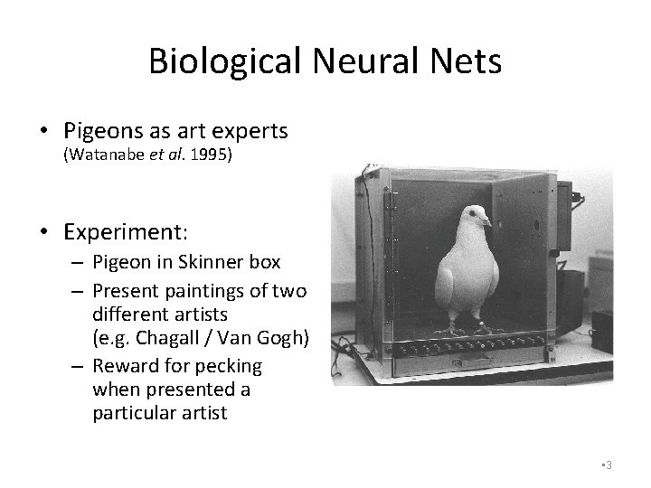
Biological Neural Nets • Pigeons as art experts (Watanabe et al. 1995) • Experiment: – Pigeon in Skinner box – Present paintings of two different artists (e. g. Chagall / Van Gogh) – Reward for pecking when presented a particular artist • 3

Pigeon-Art Experiment Results • Pigeon in-sample error of 5% – presented with pictures they had been trained on • Out of sample error of 15% – New, unseen paintings of Chagall / Van Gogh • Pigeons must be learning something (not memorization) – Extract and recognise patterns (the ‘style’) – Generalize from the already seen to make predictions • This is the idea behind neural networks (biological and artificial) • 4

Artificial Neural Networks (ANN) • Popular set of learning techniques – Popularity ebbs and flows over time – Currently in a resurgence • Common features of ANNs – Networks of simple elements – Inspired (loosely) by brain organization – Compact representation • 5

ANNs (cont’d) • Highly parallel – Process information much more like the brain than a serial computer • Simple principles complex behaviours • Applications – As powerful problem solvers – As biological models • 6

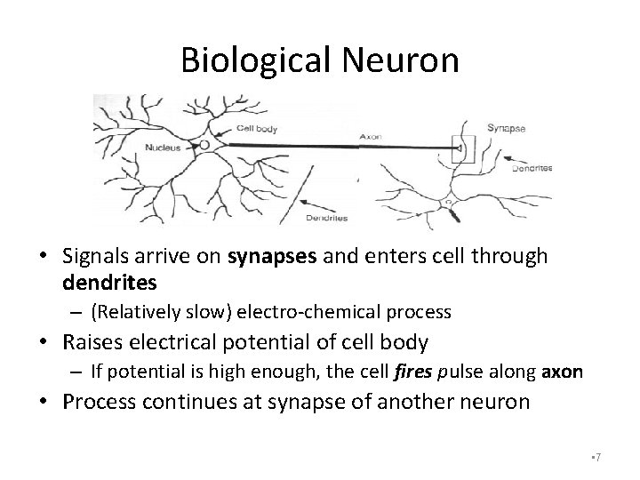
Biological Neuron • Signals arrive on synapses and enters cell through dendrites – (Relatively slow) electro-chemical process • Raises electrical potential of cell body – If potential is high enough, the cell fires pulse along axon • Process continues at synapse of another neuron • 7

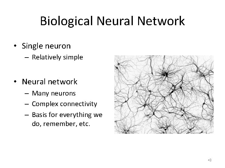
Biological Neural Network • Single neuron – Relatively simple • Neural network – Many neurons – Complex connectivity – Basis for everything we do, remember, etc. • 8

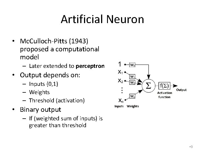
Artificial Neuron • Mc. Culloch-Pitts (1943) proposed a computational model – Later extended to perceptron • Output depends on: – Inputs {0, 1} – Weights – Threshold (activation) • Binary output – If (weighted sum of inputs) is greater than threshold • 9

Real vs Artificial Neurons • Main differences – Discrete Time – No refractory period – Real neurons use spike trains, not single signals – Real neurons are often not threshold devices – Many real cells do nonlinear summation on inputs • Some research into more accurate neuron models – However, this is mostly to more accurately model neurons and not for ANNs • 10

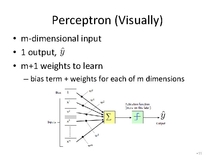
Perceptron (Visually) • m-dimensional input • 1 output, • m+1 weights to learn – bias term + weights for each of m dimensions • 11

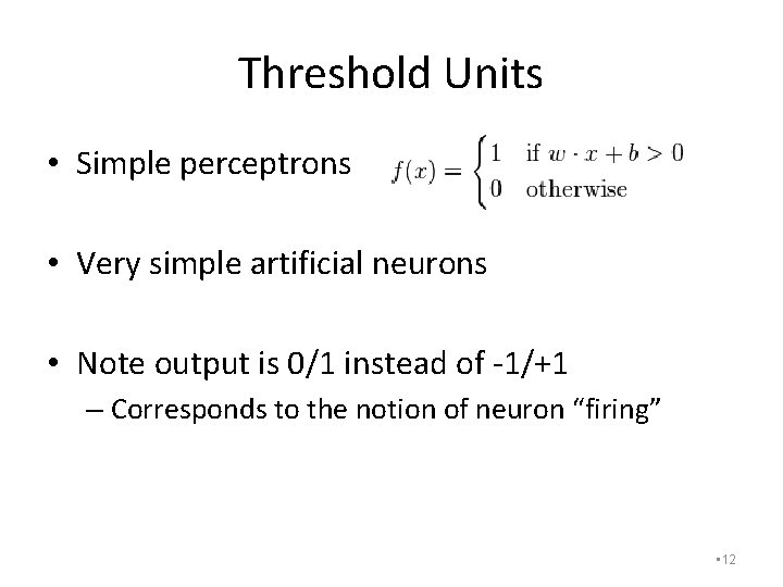
Threshold Units • Simple perceptrons • Very simple artificial neurons • Note output is 0/1 instead of -1/+1 – Corresponds to the notion of neuron “firing” • 12

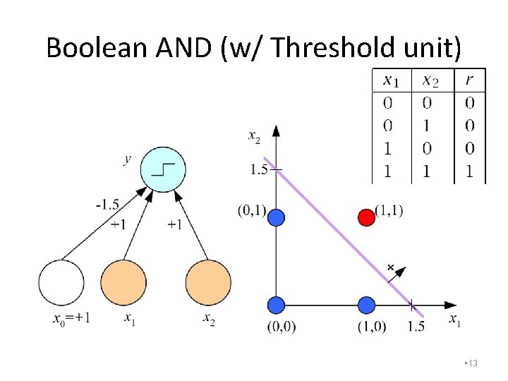
Boolean AND (w/ Threshold unit) • 13

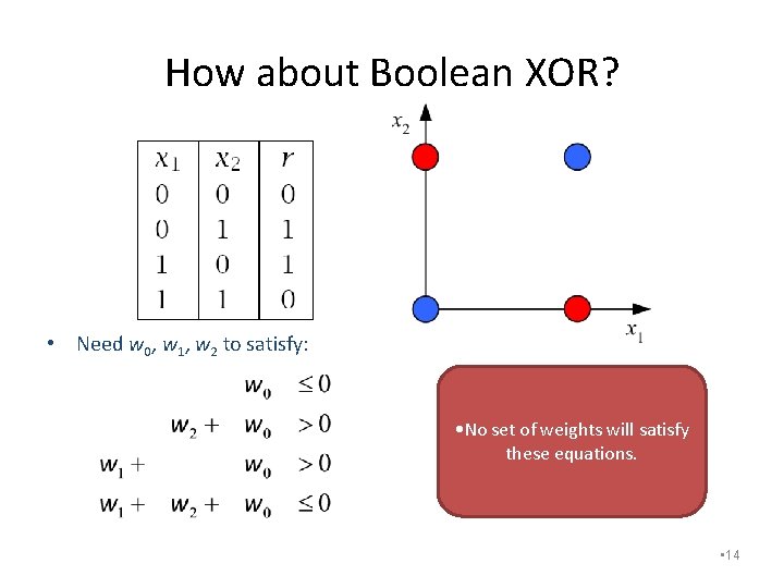
How about Boolean XOR? • Need w 0, w 1, w 2 to satisfy: • No set of weights will satisfy these equations. • 14

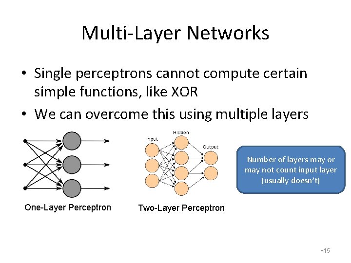
Multi-Layer Networks • Single perceptrons cannot compute certain simple functions, like XOR • We can overcome this using multiple layers Number of layers may or may not count input layer (usually doesn’t) One-Layer Perceptron Two-Layer Perceptron • 15

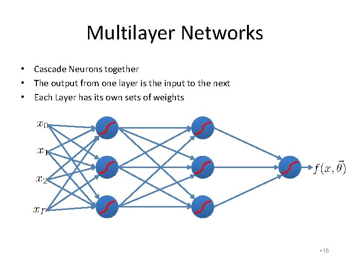
Multilayer Networks • Cascade Neurons together • The output from one layer is the input to the next • Each Layer has its own sets of weights • 16

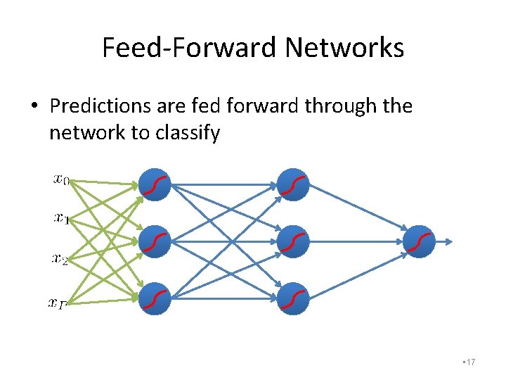
Feed-Forward Networks • Predictions are fed forward through the network to classify • 17

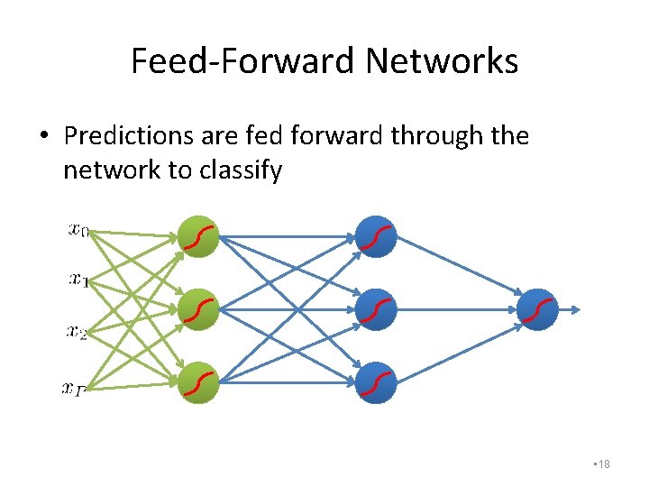
Feed-Forward Networks • Predictions are fed forward through the network to classify • 18

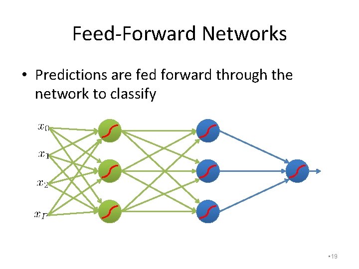
Feed-Forward Networks • Predictions are fed forward through the network to classify • 19

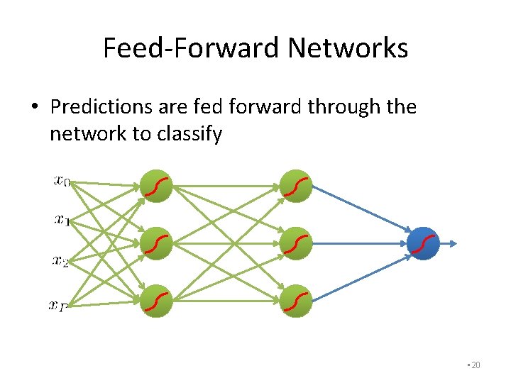
Feed-Forward Networks • Predictions are fed forward through the network to classify • 20

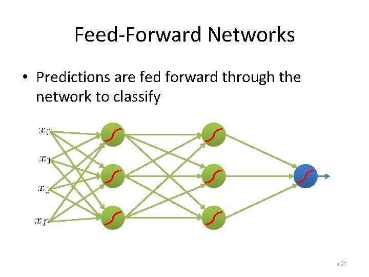
Feed-Forward Networks • Predictions are fed forward through the network to classify • 21

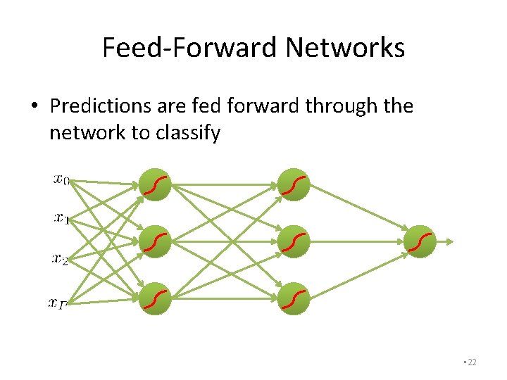
Feed-Forward Networks • Predictions are fed forward through the network to classify • 22

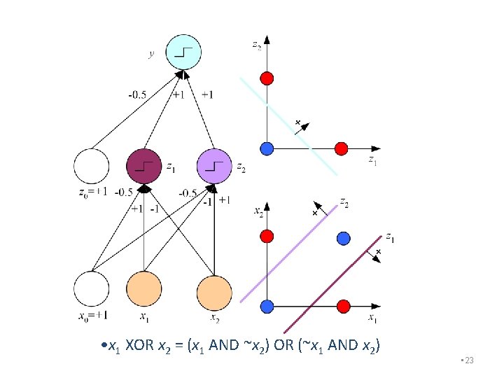
• x 1 XOR x 2 = (x 1 AND ~x 2) OR (~x 1 AND x 2) • 23

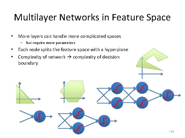
Multilayer Networks in Feature Space • More layers can handle more complicated spaces – but require more parameters • Each node splits the feature space with a hyperplane • Complexity of network complexity of decision boundary • 24

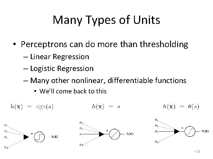
Many Types of Units • Perceptrons can do more than thresholding – Linear Regression – Logistic Regression – Many other nonlinear, differentiable functions • We’ll come back to this • 25

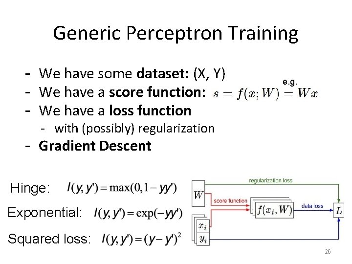
Generic Perceptron Training - We have some dataset: (X, Y) - We have a score function: - We have a loss function e. g. - with (possibly) regularization - Gradient Descent Hinge: Exponential: Squared loss: 26

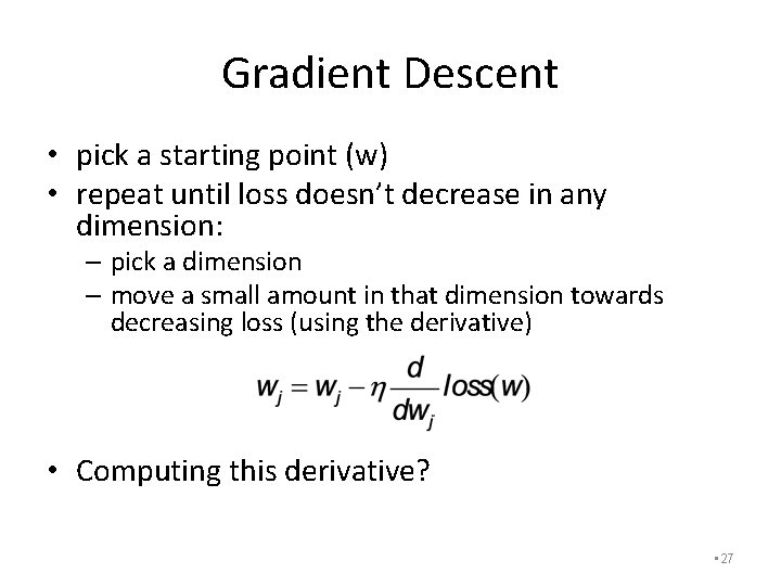
Gradient Descent • pick a starting point (w) • repeat until loss doesn’t decrease in any dimension: – pick a dimension – move a small amount in that dimension towards decreasing loss (using the derivative) • Computing this derivative? • 27

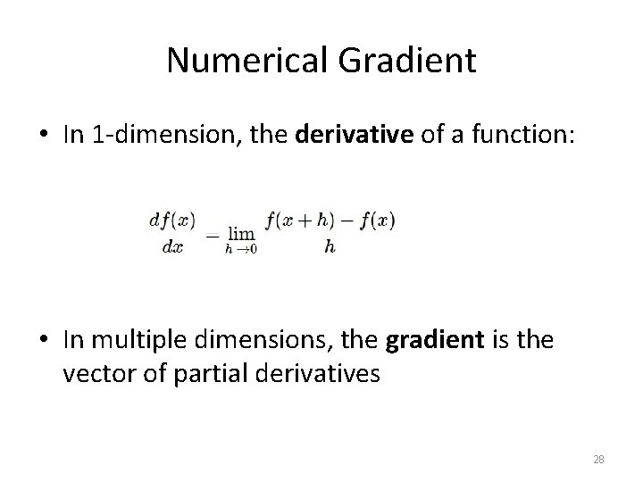
Numerical Gradient • In 1 -dimension, the derivative of a function: • In multiple dimensions, the gradient is the vector of partial derivatives 28

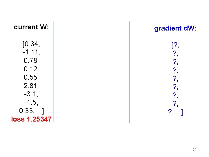
current W: gradient d. W: [0. 34, -1. 11, 0. 78, 0. 12, 0. 55, 2. 81, -3. 1, -1. 5, 0. 33, …] loss 1. 25347 [? , ? , ? , …] 29

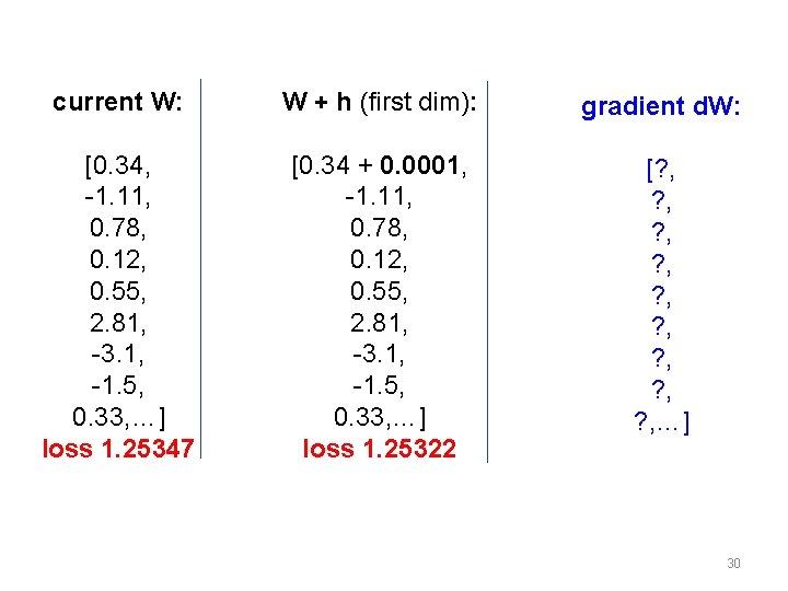
current W: W + h (first dim): gradient d. W: [0. 34, -1. 11, 0. 78, 0. 12, 0. 55, 2. 81, -3. 1, -1. 5, 0. 33, …] loss 1. 25347 [0. 34 + 0. 0001, -1. 11, 0. 78, 0. 12, 0. 55, 2. 81, -3. 1, -1. 5, 0. 33, …] loss 1. 25322 [? , ? , ? , …] 30

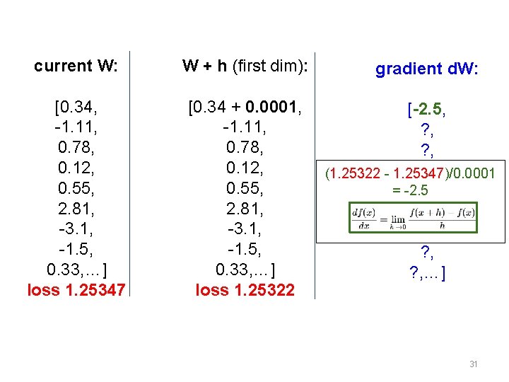
current W: W + h (first dim): [0. 34, -1. 11, 0. 78, 0. 12, 0. 55, 2. 81, -3. 1, -1. 5, 0. 33, …] loss 1. 25347 [0. 34 + 0. 0001, -1. 11, 0. 78, 0. 12, 0. 55, 2. 81, -3. 1, -1. 5, 0. 33, …] loss 1. 25322 gradient d. W: [-2. 5, ? , ? , (1. 25322 - 1. 25347)/0. 0001 = -2. 5 ? , ? , ? , …] 31

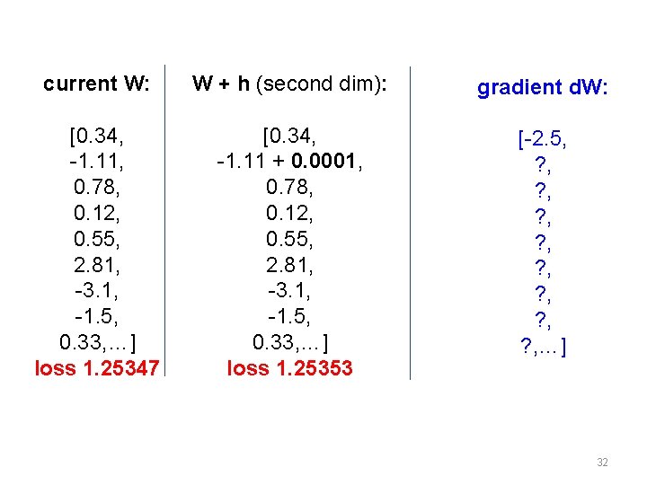
current W: W + h (second dim): gradient d. W: [0. 34, -1. 11, 0. 78, 0. 12, 0. 55, 2. 81, -3. 1, -1. 5, 0. 33, …] loss 1. 25347 [0. 34, -1. 11 + 0. 0001, 0. 78, 0. 12, 0. 55, 2. 81, -3. 1, -1. 5, 0. 33, …] loss 1. 25353 [-2. 5, ? , ? , …] 32

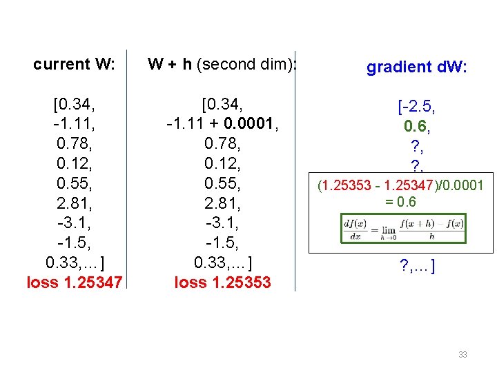
current W: W + h (second dim): [0. 34, -1. 11, 0. 78, 0. 12, 0. 55, 2. 81, -3. 1, -1. 5, 0. 33, …] loss 1. 25347 [0. 34, -1. 11 + 0. 0001, 0. 78, 0. 12, 0. 55, 2. 81, -3. 1, -1. 5, 0. 33, …] loss 1. 25353 gradient d. W: [-2. 5, 0. 6, ? , (1. 25353 - 1. 25347)/0. 0001 ? , = 0. 6? , ? , …] 33

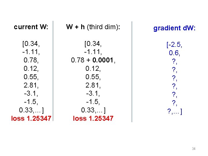
current W: W + h (third dim): gradient d. W: [0. 34, -1. 11, 0. 78, 0. 12, 0. 55, 2. 81, -3. 1, -1. 5, 0. 33, …] loss 1. 25347 [0. 34, -1. 11, 0. 78 + 0. 0001, 0. 12, 0. 55, 2. 81, -3. 1, -1. 5, 0. 33, …] loss 1. 25347 [-2. 5, 0. 6, ? , ? , …] 34

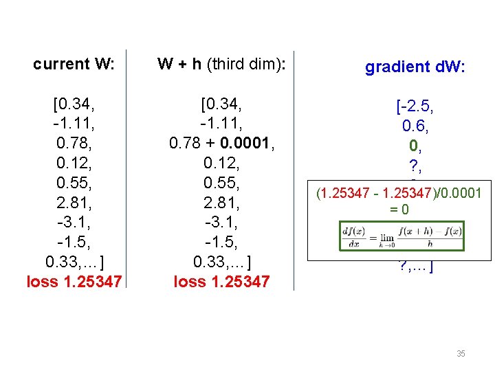
current W: W + h (third dim): [0. 34, -1. 11, 0. 78, 0. 12, 0. 55, 2. 81, -3. 1, -1. 5, 0. 33, …] loss 1. 25347 [0. 34, -1. 11, 0. 78 + 0. 0001, 0. 12, 0. 55, 2. 81, -3. 1, -1. 5, 0. 33, …] loss 1. 25347 gradient d. W: [-2. 5, 0. 6, 0, ? , (1. 25347 - 1. 25347)/0. 0001 = 0? , ? , …] 35

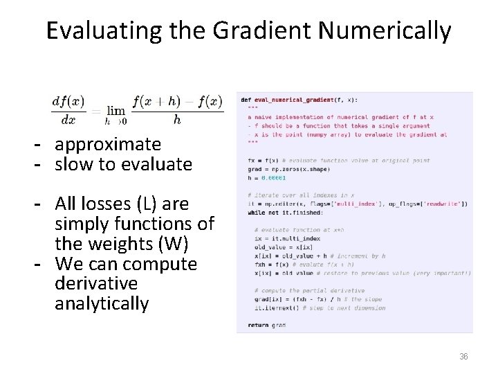
Evaluating the Gradient Numerically - approximate - slow to evaluate - All losses (L) are simply functions of the weights (W) - We can compute derivative analytically 36

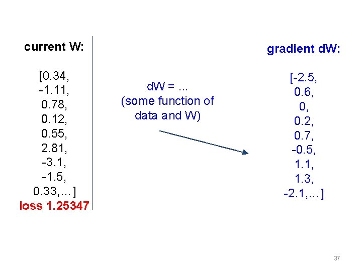
current W: gradient d. W: [0. 34, -1. 11, 0. 78, 0. 12, 0. 55, 2. 81, -3. 1, -1. 5, 0. 33, …] loss 1. 25347 [-2. 5, 0. 6, 0, 0. 2, 0. 7, -0. 5, 1. 1, 1. 3, -2. 1, …] d. W =. . . (some function of data and W) 37

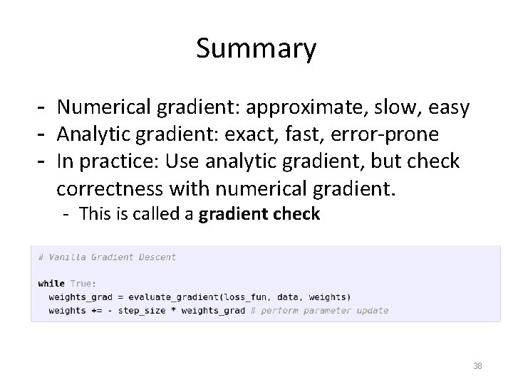
Summary - Numerical gradient: approximate, slow, easy - Analytic gradient: exact, fast, error-prone - In practice: Use analytic gradient, but check correctness with numerical gradient. - This is called a gradient check 38

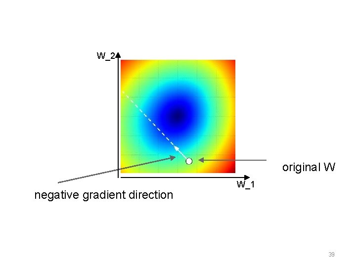
W_2 original W negative gradient direction W_1 39

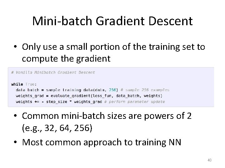
Mini-batch Gradient Descent • Only use a small portion of the training set to compute the gradient • Common mini-batch sizes are powers of 2 (e. g. , 32, 64, 256) • Most common approach to training NN 40

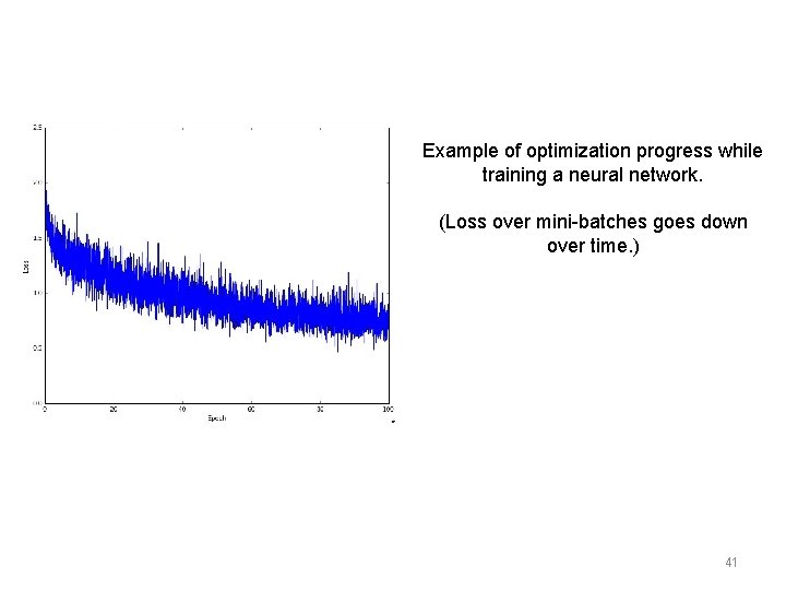
Example of optimization progress while training a neural network. (Loss over mini-batches goes down over time. ) 41

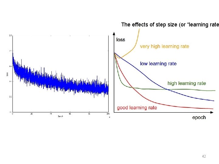
The effects of step size (or “learning rate 42

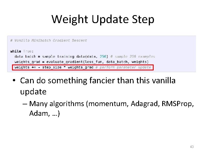
Weight Update Step • Can do something fancier than this vanilla update – Many algorithms (momentum, Adagrad, RMSProp, Adam, …) 43

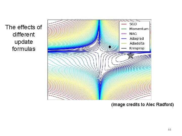
The effects of different update formulas (image credits to Alec Radford) 44

What do we have so far… • Components – biological plausibility – Neuron / node – Synapses / weight • Perceptrons / Artificial Neurons – Threshold Units (boolean functions / classification) – Linear Units (regression) – Nonlinear Units • Similarities across units… – All can be trained via gradient descent – Weights of the connections between nodes determine the behavior of a unit or network • 45

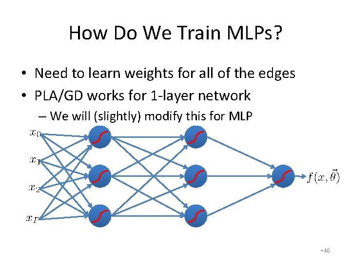
How Do We Train MLPs? • Need to learn weights for all of the edges • PLA/GD works for 1 -layer network – We will (slightly) modify this for MLP • 46

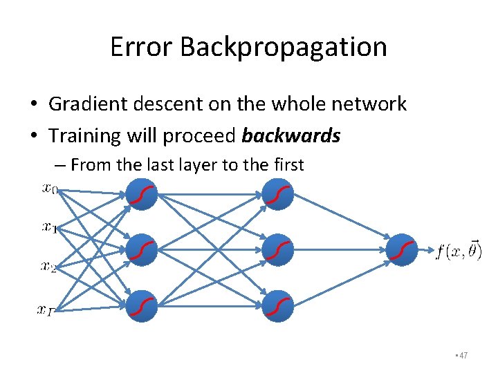
Error Backpropagation • Gradient descent on the whole network • Training will proceed backwards – From the last layer to the first • 47

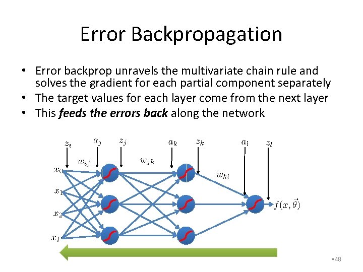
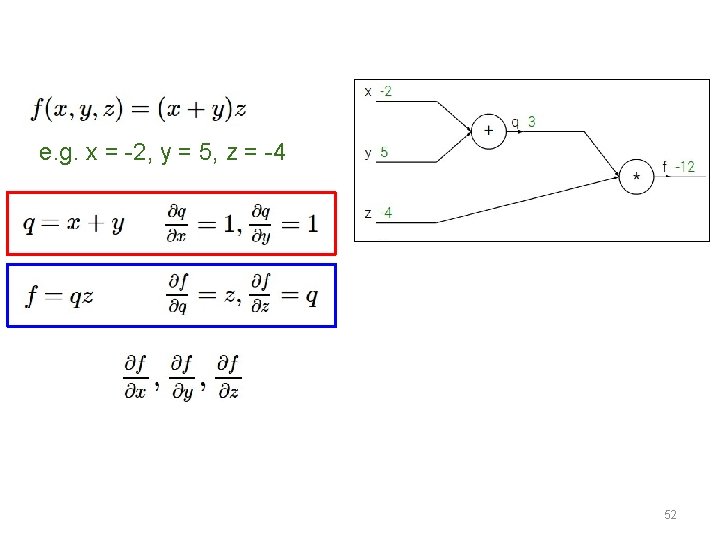
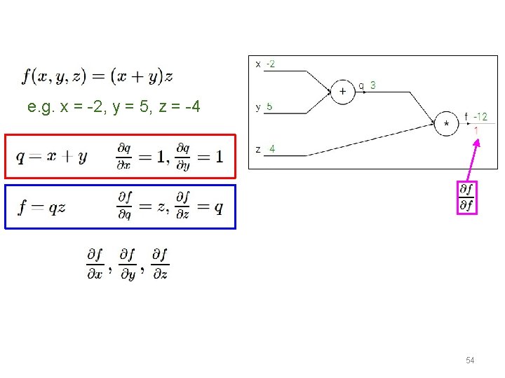
Error Backpropagation • Error backprop unravels the multivariate chain rule and solves the gradient for each partial component separately • The target values for each layer come from the next layer • This feeds the errors back along the network • 48

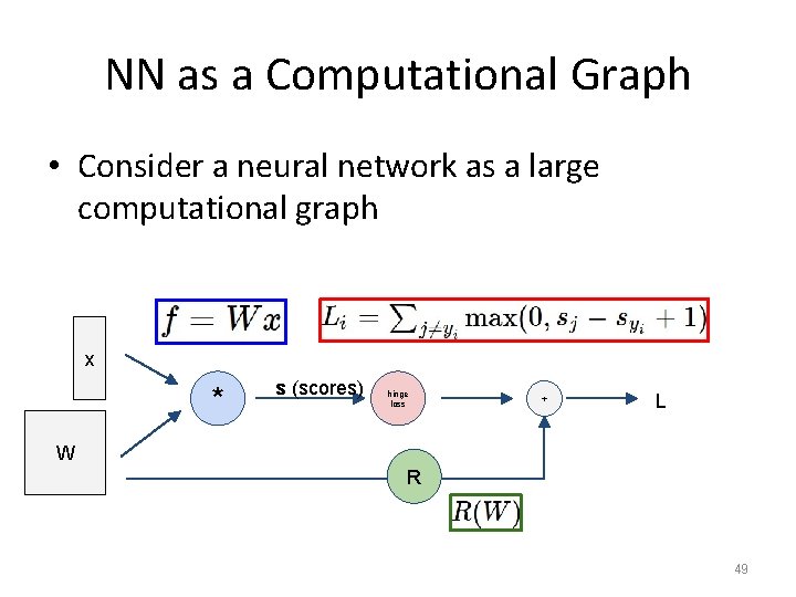
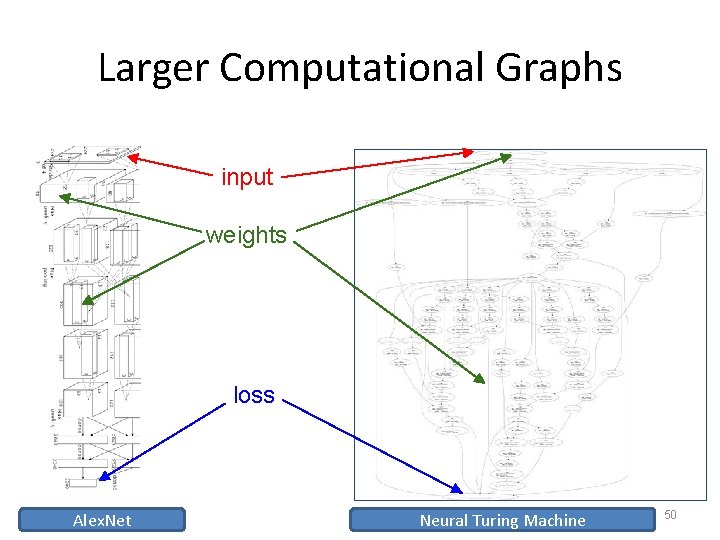
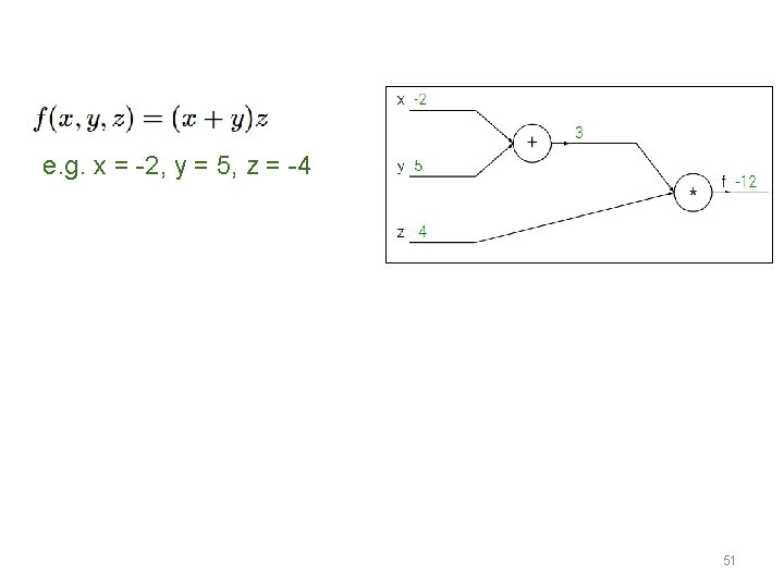
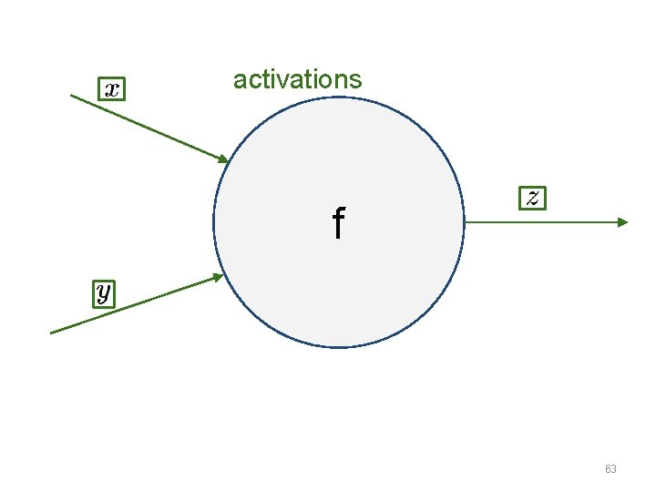
NN as a Computational Graph • Consider a neural network as a large computational graph x * s (scores) hinge loss + L W R 49

Larger Computational Graphs input weights loss Alex. Net Neural Turing Machine 50

e. g. x = -2, y = 5, z = -4 51

e. g. x = -2, y = 5, z = -4 Want: 52

e. g. x = -2, y = 5, z = -4 Want: 53

e. g. x = -2, y = 5, z = -4 Want: 54

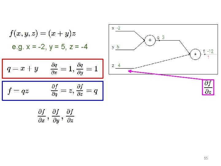
e. g. x = -2, y = 5, z = -4 Want: 55

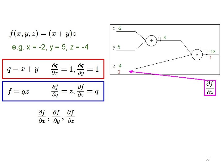
e. g. x = -2, y = 5, z = -4 Want: 56

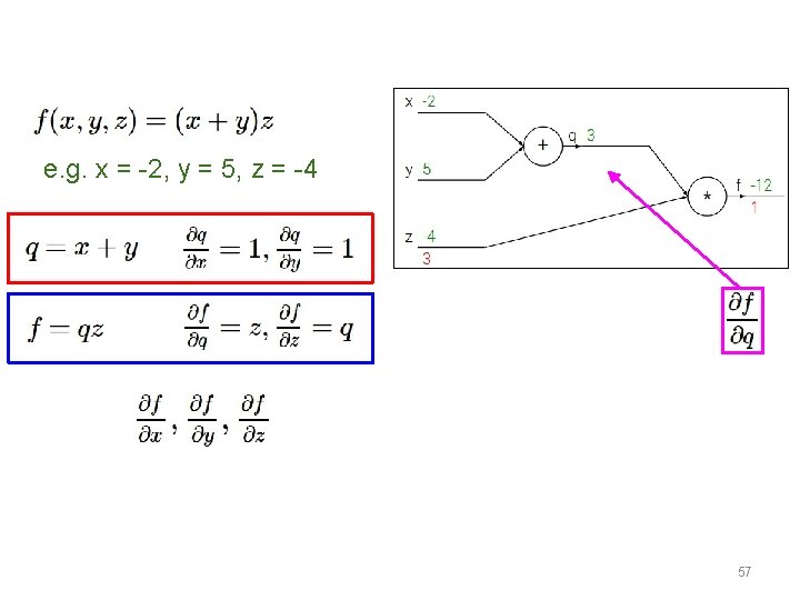
e. g. x = -2, y = 5, z = -4 Want: 57

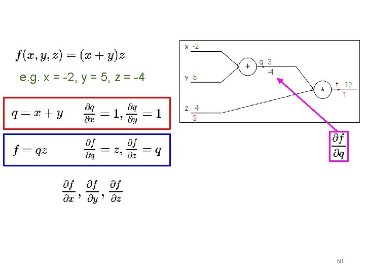
e. g. x = -2, y = 5, z = -4 Want: 58

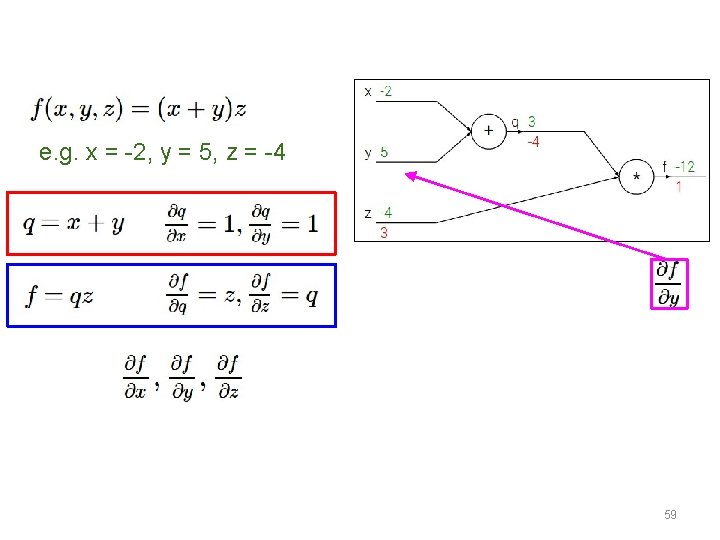
e. g. x = -2, y = 5, z = -4 Want: 59

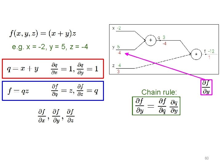
e. g. x = -2, y = 5, z = -4 Chain rule: Want: 60

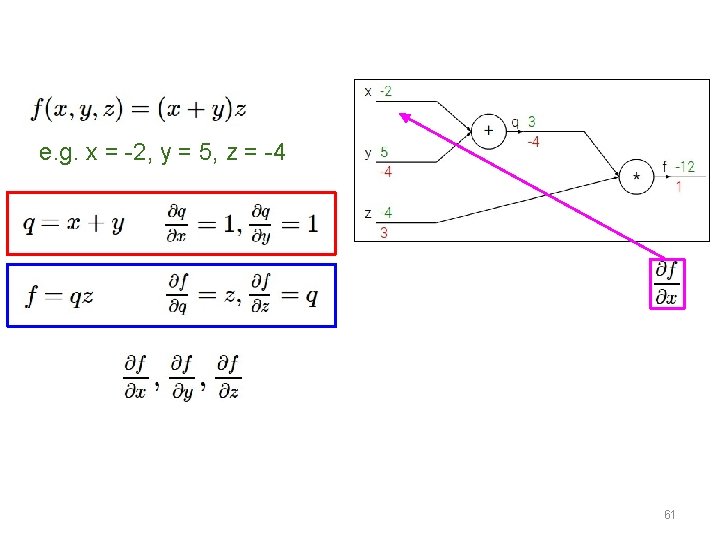
e. g. x = -2, y = 5, z = -4 Want: 61

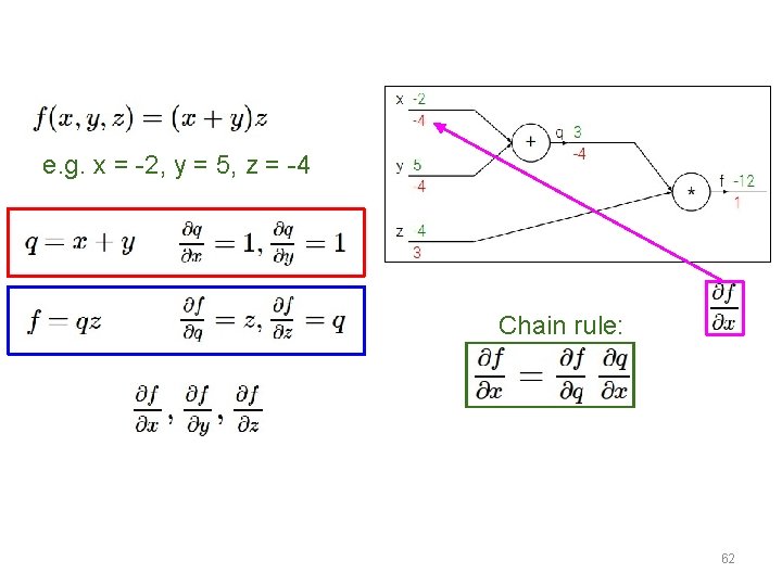
e. g. x = -2, y = 5, z = -4 Chain rule: Want: 62

activations f 63

activations “local gradient” f 64

activations “local gradient” f gradien 65

activations “local gradient” f gradien 66

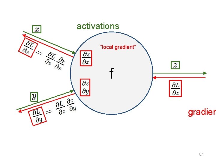
activations “local gradient” f gradien 67

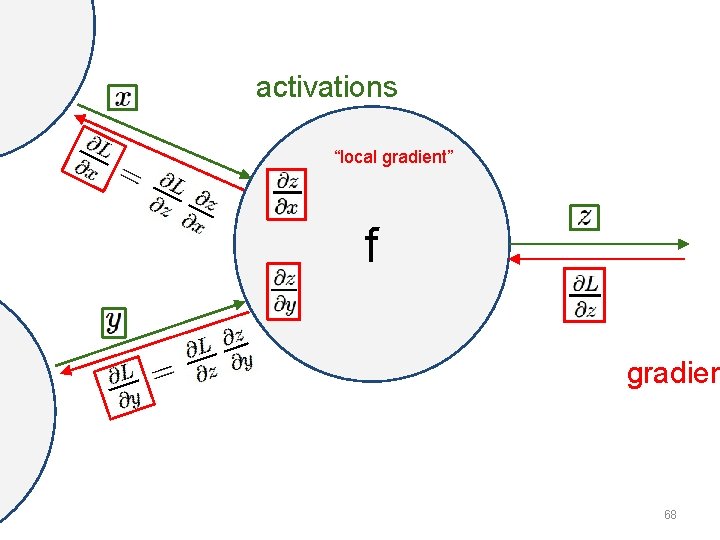
activations “local gradient” f gradien 68

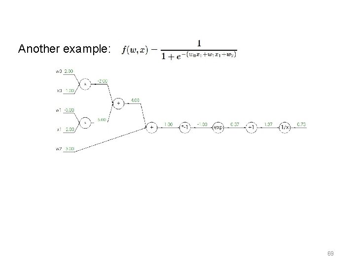
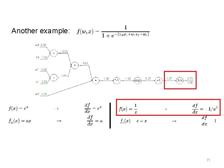
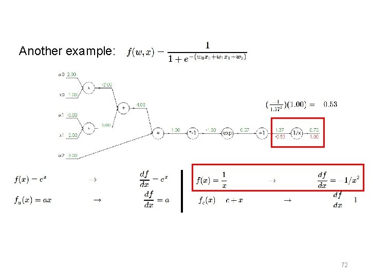
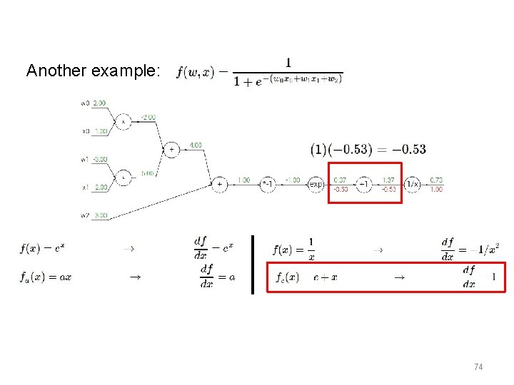
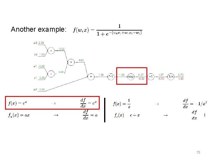
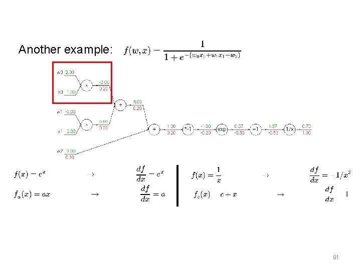
Another example: 69

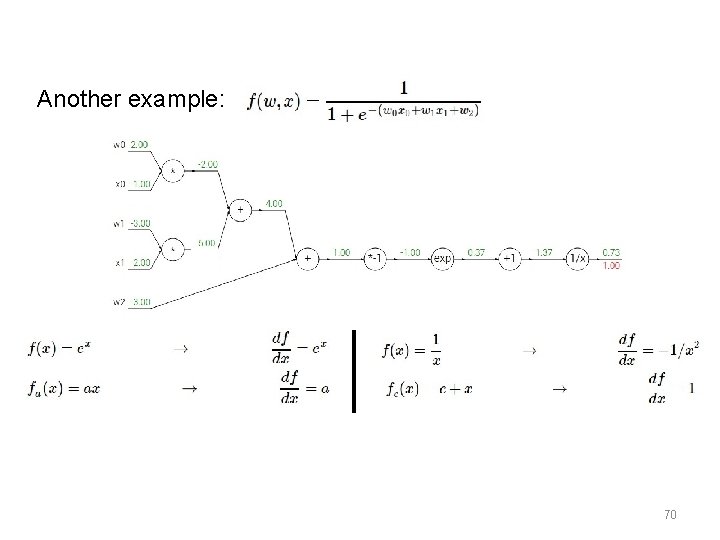
Another example: 70

Another example: 71

Another example: 72

Another example: 73

Another example: 74

Another example: 75

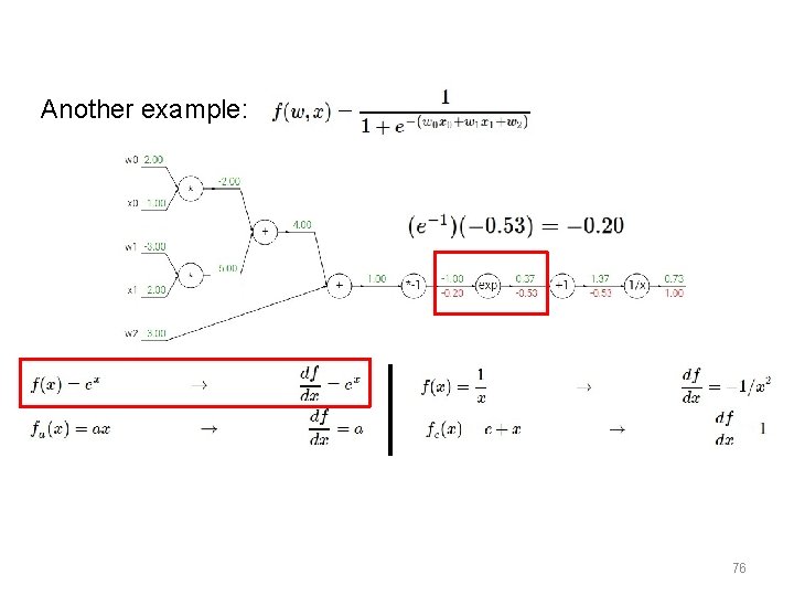
Another example: 76

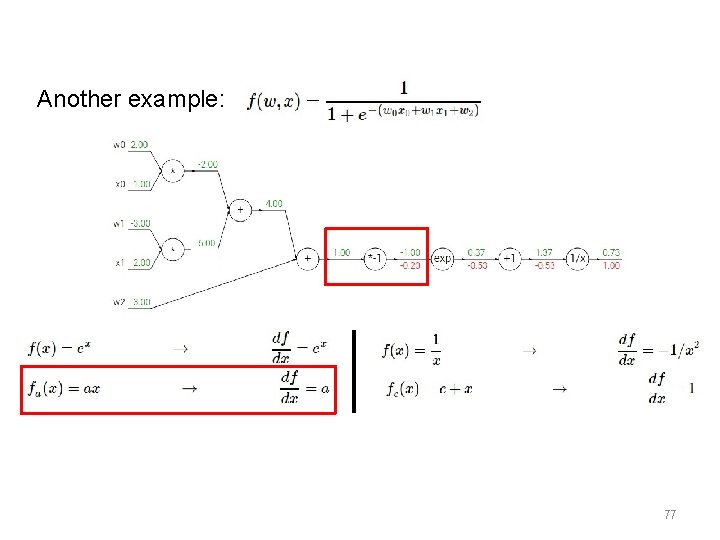
Another example: 77

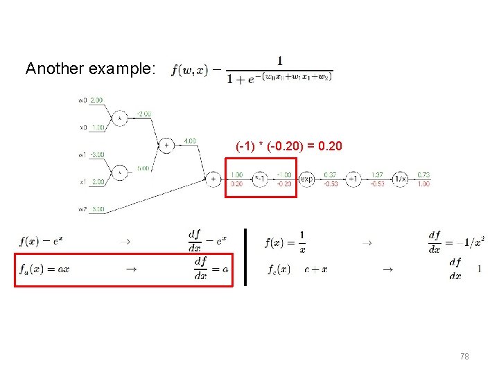
Another example: (-1) * (-0. 20) = 0. 20 78

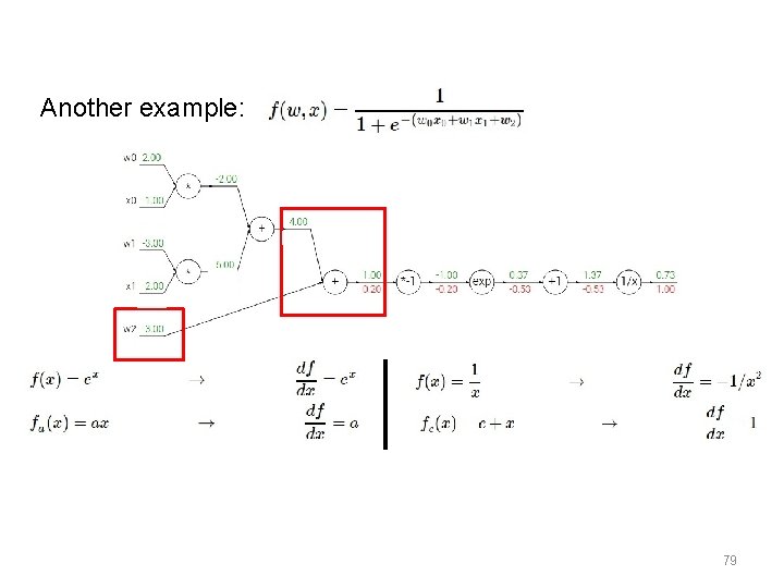
Another example: 79

Another example: [local gradient] x [its gradient] [1] x [0. 2] = 0. 2 (both inputs!) 80

Another example: 81

Another example: [local gradient] x [its gradient] x 0: [2] x [0. 2] = 0. 4 w 0: [-1] x [0. 2] = -0. 2 82

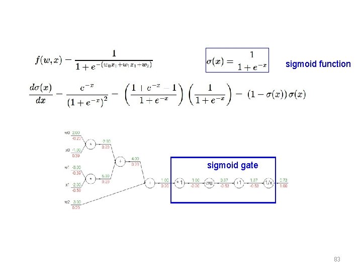
sigmoid function sigmoid gate 83

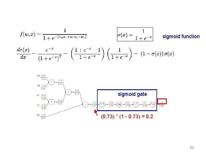
sigmoid function sigmoid gate (0. 73) * (1 - 0. 73) = 0. 2 84

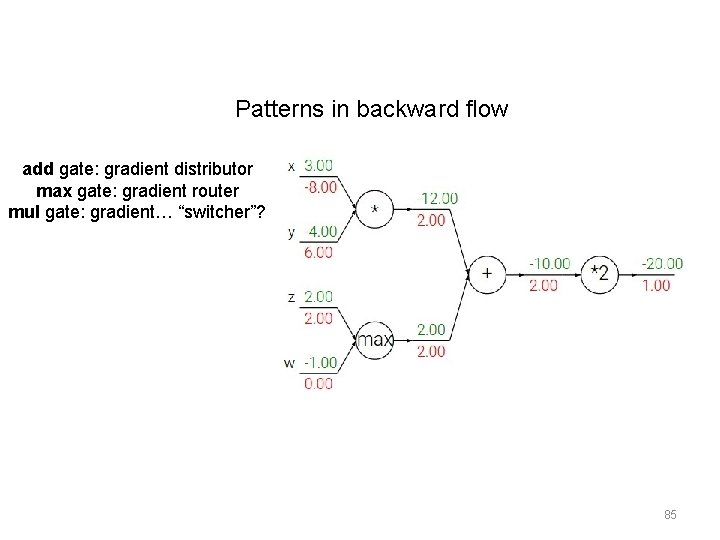
Patterns in backward flow add gate: gradient distributor max gate: gradient router mul gate: gradient… “switcher”? 85

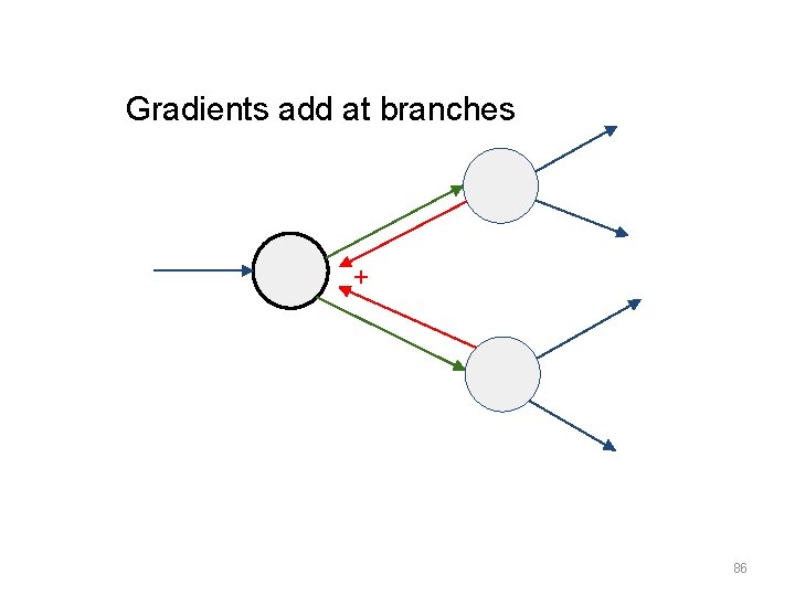
Gradients add at branches + 86

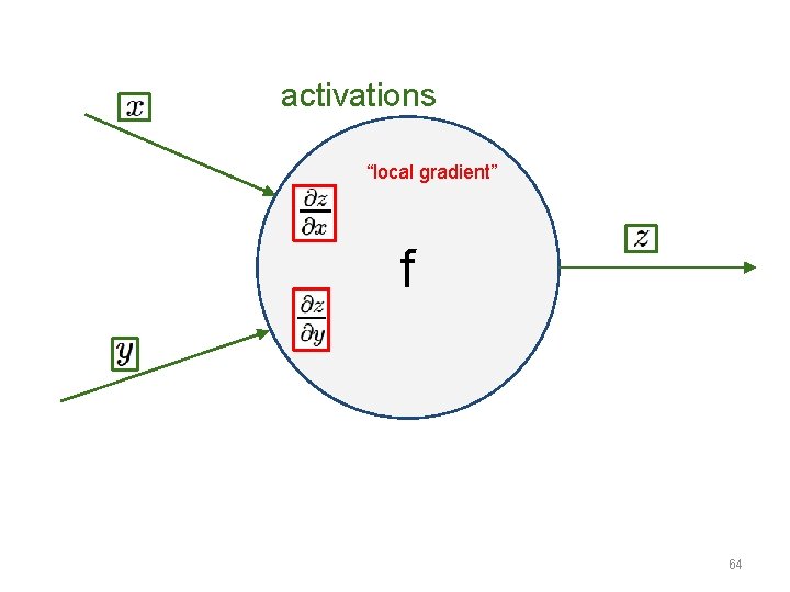
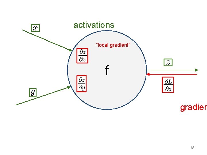
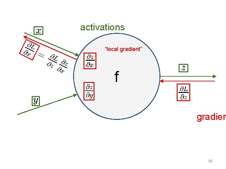
Backprop Summary - Modern neural nets are very large - No hope of writing down gradient formula by hand for all parameters - Backpropagation: recursive application of the chain rule along a computational graph to compute the gradients of all inputs/parameters/intermediates - Should maintain a graph structure, where the nodes implement forward() and backward() - forward: compute result of an operation and save any intermediates needed for gradient computation in memory - backward: apply the chain rule to compute the gradient of the loss function with respect to the inputs 87

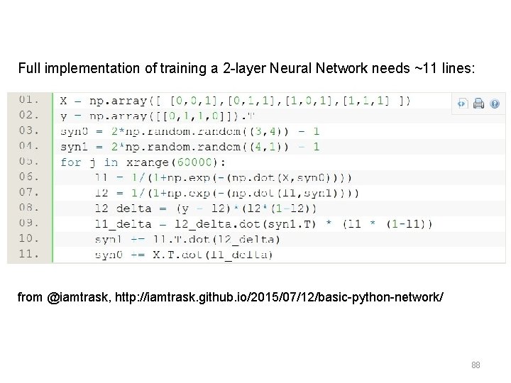
Full implementation of training a 2 -layer Neural Network needs ~11 lines: from @iamtrask, http: //iamtrask. github. io/2015/07/12/basic-python-network/ 88

How does this work in practice? 1. Initialize all weights to small, non-zero values 2. Choose a training point (or mini-batch) and clamp to input layer 3. Propagate signal forward thru network until output is generated 4. Calculate deltas for output layer • 89

Backprop. in practice (cont’d) 5. Calculate deltas for previous layers by propagating errors backwards until a delta is calculated for every unit 6. Calculate weight updates for every weight 7. Update weights (using some update strategy) 8. Goto step 2 • 90

Notes on Backpropagation • Learning is incremental – Training examples will be presented multiple times – Especially with small learning rates • This is very basic backprop. – Other error functions – Momentum – Different learning rules • Backprop. will only find local minima • In practice, it works better with: – inputs in the range [-1, +1] – small weights • 91

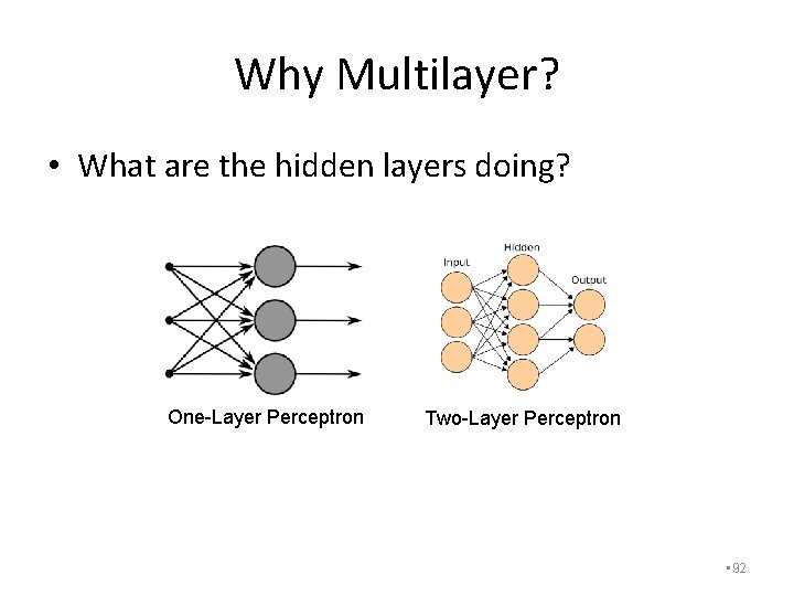
Why Multilayer? • What are the hidden layers doing? One-Layer Perceptron Two-Layer Perceptron • 92

Feature / Representation Learning • Each layer maps input to a new feature space – You can get away with less clever feature representations using MLP – At what cost? • Increased VC dimension (also MLP prone to overfitting) • Nonlinearities can make interpretation of the hidden layers very difficult • Often, MLPs are treated as black boxes • 93

Other Neural Networks • Backprop generalizes to networks that skip layers • Many variants of ANN – Multiple Outputs – Skip Layer Network – Recurrent Neural Networks • 94

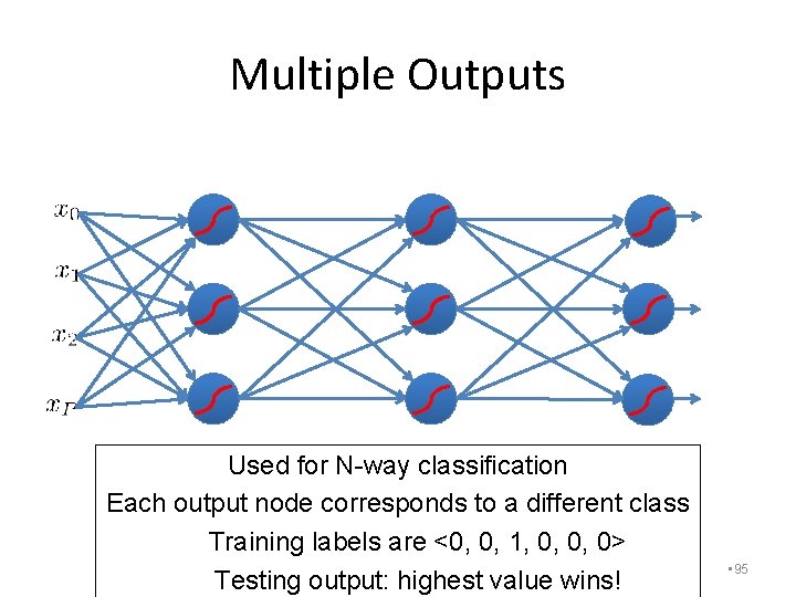
Multiple Outputs Used for N-way classification Each output node corresponds to a different class Training labels are <0, 0, 1, 0, 0, 0> Testing output: highest value wins! • 95

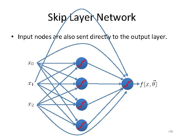
Skip Layer Network • Input nodes are also sent directly to the output layer. • 96

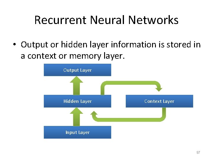
Recurrent Neural Networks • Output or hidden layer information is stored in a context or memory layer. Output Layer Hidden Layer Context Layer Input Layer 97

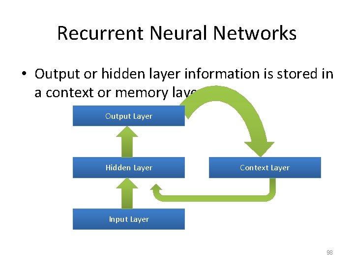
Recurrent Neural Networks • Output or hidden layer information is stored in a context or memory layer. Output Layer Hidden Layer Context Layer Input Layer 98

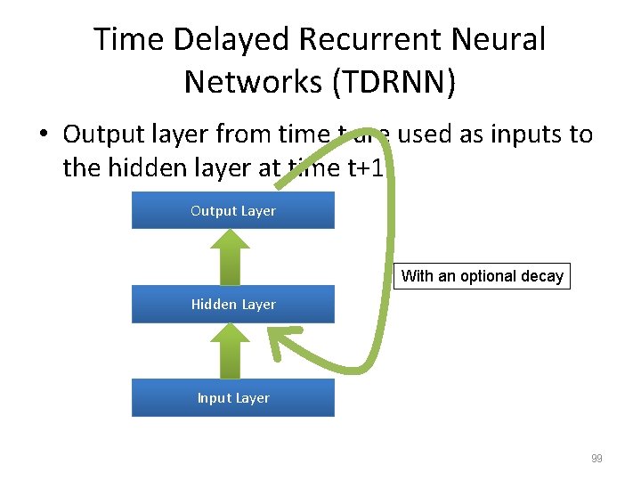
Time Delayed Recurrent Neural Networks (TDRNN) • Output layer from time t are used as inputs to the hidden layer at time t+1. Output Layer With an optional decay Hidden Layer Input Layer 99

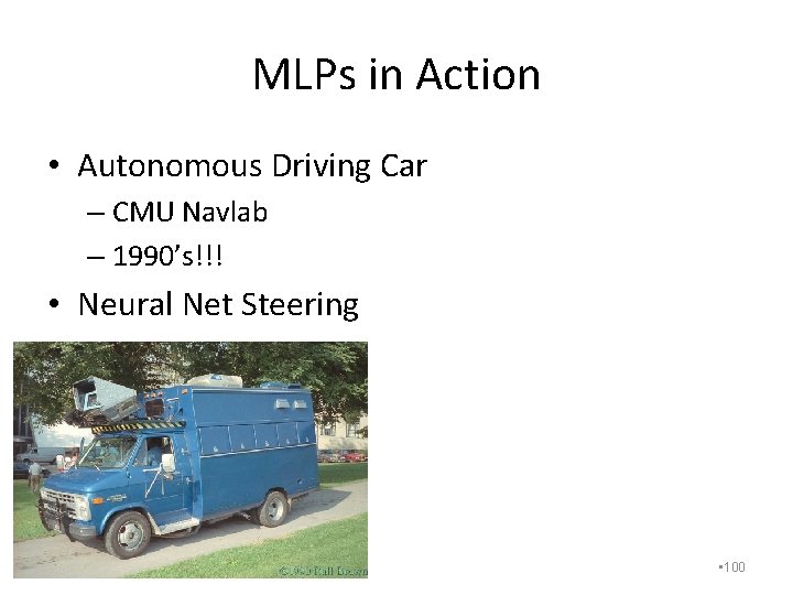
MLPs in Action • Autonomous Driving Car – CMU Navlab – 1990’s!!! • Neural Net Steering • 100

Artificial Neural Networks • MLPs are a network of simple units – Lead to complex learners • Error backpropagation trains an MLP – Gradient descent applied to entire network – Trains network “one layer at a time” • These types of MLPs are usually ≤ 3 layers – Vanishing gradients – Too many params • Next Time: Deep Learning • 101