Artificial neural networks ANNs The neuron model The

Artificial neural networks (ANNs)

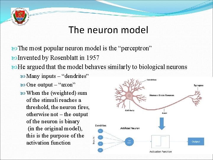
The neuron model The most popular neuron model is the “perceptron” Invented by Rosenblatt in 1957 He argued that the model behaves similarly to biological neurons Many inputs – “dendrites” One output – “axon” When the (weighted) sum of the stimuli reaches a threshold, the neuron fires, otherwise not – the output of the neuron is binary (in the original model), this is the purpose of the activation function

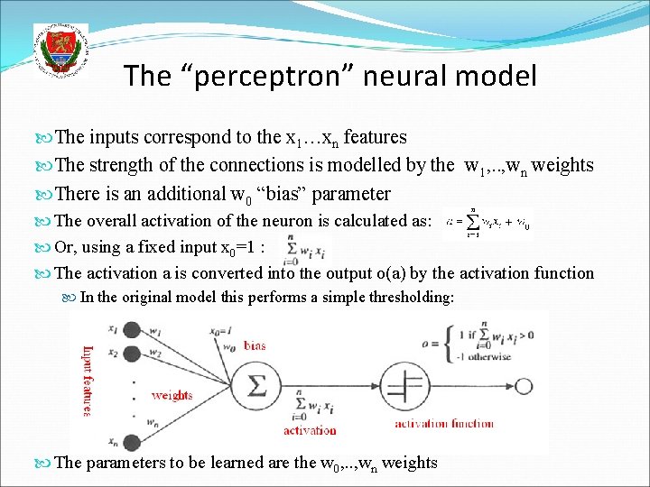
The “perceptron” neural model The inputs correspond to the x 1…xn features The strength of the connections is modelled by the w 1, . . , wn weights There is an additional w 0 “bias” parameter The overall activation of the neuron is calculated as: Or, using a fixed input x 0=1 : The activation a is converted into the output o(a) by the activation function In the original model this performs a simple thresholding: The parameters to be learned are the w 0, . . , wn weights

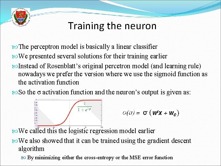
Training the neuron The perceptron model is basically a linear classifier We presented several solutions for their training earlier Instead of Rosenblatt’s original percetron model (and learning rule) nowadays we prefer the version where we use the sigmoid function as the activation function So the σ activation function and the neuron’s output is given as: We called this the logistic regression model earlier We also showed that it can be trained using the gradient descent algorithm By minimizing either the cross-entropy or the MSE error function

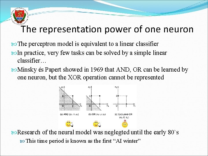
The representation power of one neuron The perceptron model is equivalent to a linear classifier In practice, very few tasks can be solved by a simple linear classifier… Minsky és Papert showed in 1969 that AND, OR can be learned by one neuron, but the XOR operation cannot be represented Research of the neural model was neglegted until the early 80`s This time period is known as the first “AI winter”

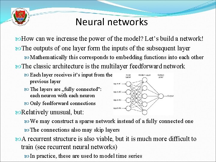
Neural networks How can we increase the power of the model? Let’s build a network! The outputs of one layer form the inputs of the subsequent layer Mathematically this corresponds to embedding functions into each other The classic architecture is the multilayer feedforward network Each layer receives it’s input from the previous layer The layers are „fully connected”: each neuron with each neuron Only feedforward connections Relatively unusual, but: We may construct a sparse network instead of a fully connected one The connections also may skip layers A recurrent structure is also viable, but it is much more difficult to train (see recurrent neural networks) In practice, these are used to model time series

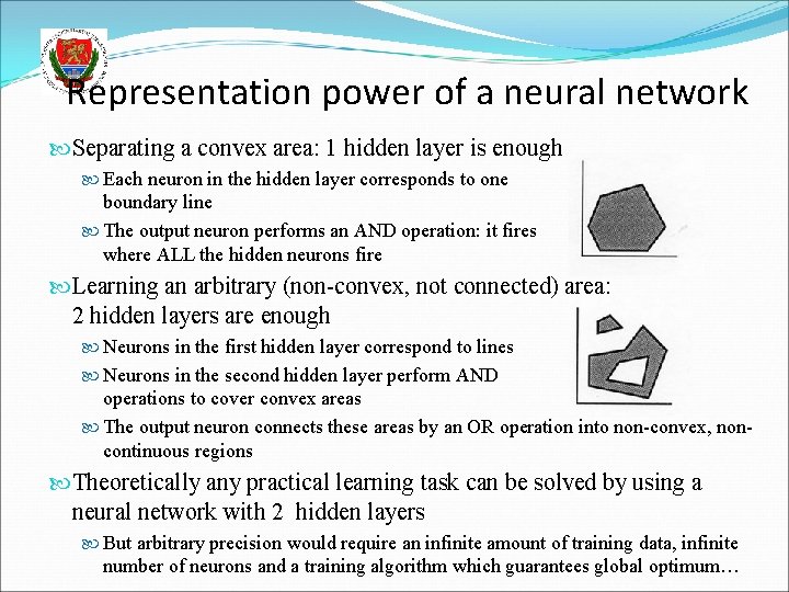
Representation power of a neural network Separating a convex area: 1 hidden layer is enough Each neuron in the hidden layer corresponds to one boundary line The output neuron performs an AND operation: it fires where ALL the hidden neurons fire Learning an arbitrary (non-convex, not connected) area: 2 hidden layers are enough Neurons in the first hidden layer correspond to lines Neurons in the second hidden layer perform AND operations to cover convex areas The output neuron connects these areas by an OR operation into non-convex, noncontinuous regions Theoretically any practical learning task can be solved by using a neural network with 2 hidden layers But arbitrary precision would require an infinite amount of training data, infinite number of neurons and a training algorithm which guarantees global optimum…

Connection with statistical pattern recognition The previous slide showed how can a network separate the classes (geometrical view) But it can also be showed that the operation of the network also can be interpreted by the decision theoretic view under certain conditions We assign an output neuron to each ci class We expect these to approximate P(ci|x) of the given class Using the outputs, we classify a given input using Bayes’ decision rule We select class ci with the largest P(ci|x) output value The proof that ANNs can approximate the P(ci|x) values required by Bayes’ decision theory increased their popularity in certain areas Knowing the P(ci|x) probabilities can be used not only for classification (by selecting the most probable class), but also for several other purposes Eg. as a confidence measue of how much the given output is reliable

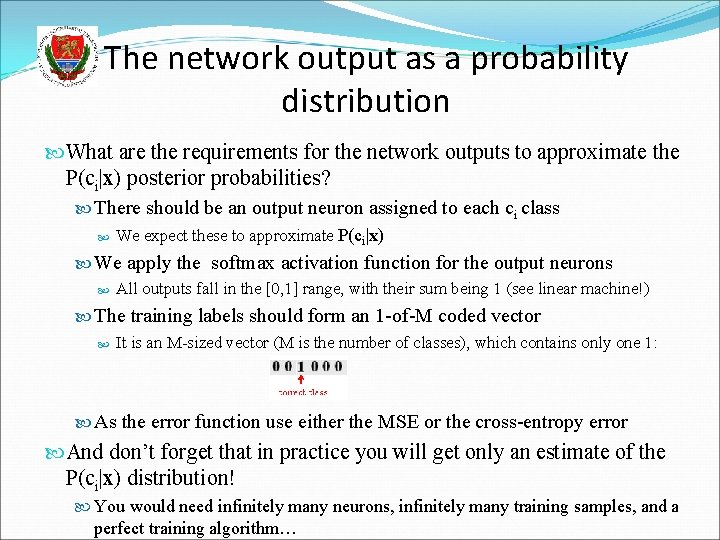
The network output as a probability distribution What are the requirements for the network outputs to approximate the P(ci|x) posterior probabilities? There should be an output neuron assigned to each ci class We expect these to approximate P(ci|x) We apply the softmax activation function for the output neurons All outputs fall in the [0, 1] range, with their sum being 1 (see linear machine!) The training labels should form an 1 -of-M coded vector It is an M-sized vector (M is the number of classes), which contains only one 1: As the error function use either the MSE or the cross-entropy error And don’t forget that in practice you will get only an estimate of the P(ci|x) distribution! You would need infinitely many neurons, infinitely many training samples, and a perfect training algorithm…

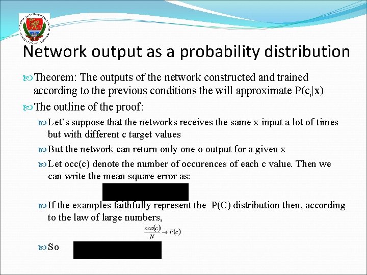
Network output as a probability distribution Theorem: The outputs of the network constructed and trained according to the previous conditions the will approximate P(ci|x) The outline of the proof: Let’s suppose that the networks receives the same x input a lot of times but with different c target values But the network can return only one o output for a given x Let occ(c) denote the number of occurences of each c value. Then we can write the mean square error as: If the examples faithfully represent the P(C) distribution then, according to the law of large numbers, So

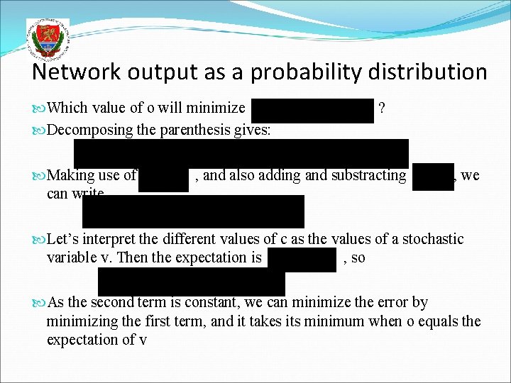
Network output as a probability distribution Which value of o will minimize Decomposing the parenthesis gives: Making use of can write ? , and also adding and substracting , we Let’s interpret the different values of c as the values of a stochastic variable v. Then the expectation is , so As the second term is constant, we can minimize the error by minimizing the first term, and it takes its minimum when o equals the expectation of v

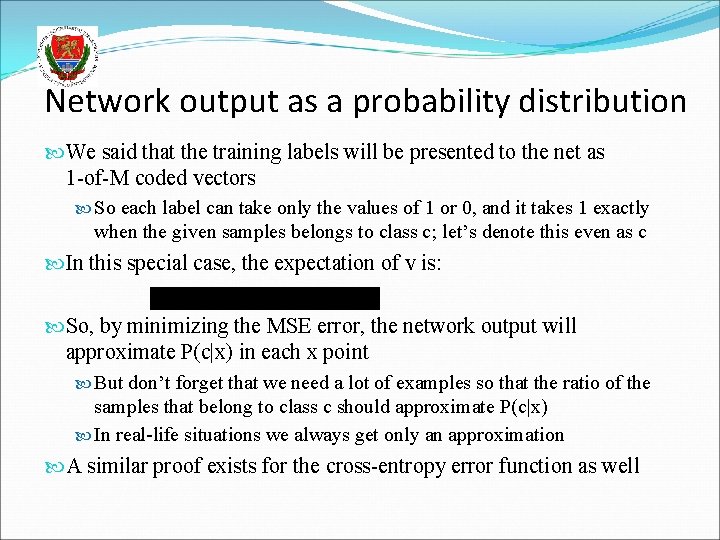
Network output as a probability distribution We said that the training labels will be presented to the net as 1 -of-M coded vectors So each label can take only the values of 1 or 0, and it takes 1 exactly when the given samples belongs to class c; let’s denote this even as c In this special case, the expectation of v is: So, by minimizing the MSE error, the network output will approximate P(c|x) in each x point But don’t forget that we need a lot of examples so that the ratio of the samples that belong to class c should approximate P(c|x) In real-life situations we always get only an approximation A similar proof exists for the cross-entropy error function as well

Training the neural network A ”network” consisting of just one neuron is equivalent with the logistic regression model presented earlier We also saw that we can train this model using the gradient descent algorithm, using either the MSE or CE error function In the multi-class case we put one neuron for each class in the output layer, and in this case we can apply multi-class logistic regression (also presented earlier) The real novelty here is when we build a multi-layer network. In this case the output of the lower layers form the input of the upper layers, which mathematically corresponds to a function embedding The gradient descent algorithm is still applicable, but the error must be propagated back from the upper layers to the lower layers This is the so-called backpropagation algorithm

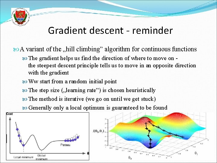
Gradient descent - reminder A variant of the „hill climbing” algorithm for continuous functions The gradient helps us find the direction of where to move on - the steepest descent principle tells us to move in an opposite direction with the gradient Ww start from a random initial point The step size („learning rate”) is chosen heuristically The method is iterative (we go on until we get stuck) Generally only a local optimum is guaranteed to be found

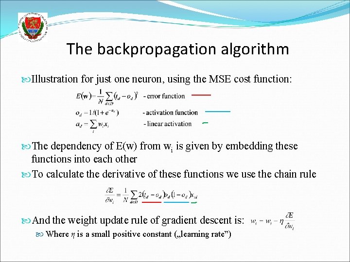
The backpropagation algorithm Illustration for just one neuron, using the MSE cost function: The dependency of E(w) from wi is given by embedding these functions into each other To calculate the derivative of these functions we use the chain rule And the weight update rule of gradient descent is: Where η is a small positive constant („learning rate”)

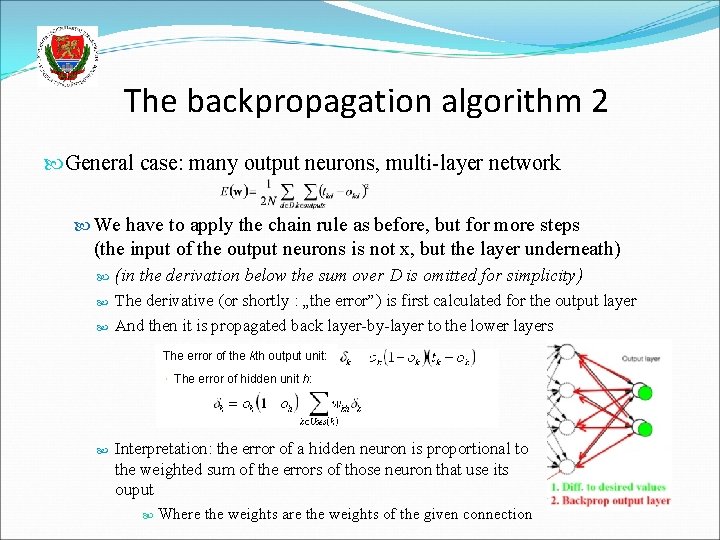
The backpropagation algorithm 2 General case: many output neurons, multi-layer network We have to apply the chain rule as before, but for more steps (the input of the output neurons is not x, but the layer underneath) (in the derivation below the sum over D is omitted for simplicity) The derivative (or shortly : „the error”) is first calculated for the output layer And then it is propagated back layer-by-layer to the lower layers The error of the kth output unit: The error of hidden unit h: Interpretation: the error of a hidden neuron is proportional to the weighted sum of the errors of those neuron that use its ouput Where the weights are the weights of the given connection

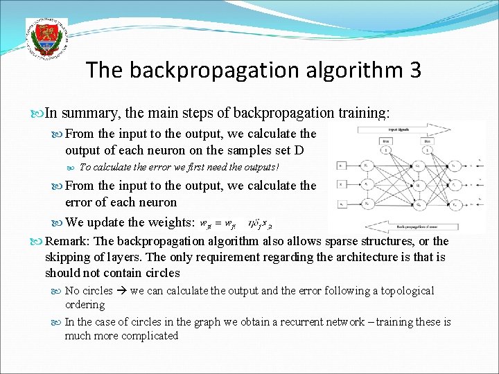
The backpropagation algorithm 3 In summary, the main steps of backpropagation training: From the input to the output, we calculate the output of each neuron on the samples set D To calculate the error we first need the outputs! From the input to the output, we calculate the error of each neuron We update the weights: Remark: The backpropagation algorithm also allows sparse structures, or the skipping of layers. The only requirement regarding the architecture is that is should not contain circles No circles we can calculate the output and the error following a topological ordering In the case of circles in the graph we obtain a recurrent network – training these is much more complicated

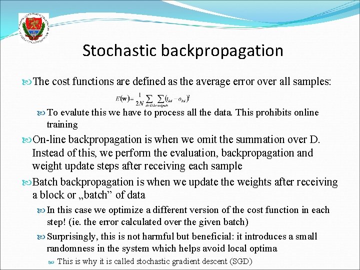
Stochastic backpropagation The cost functions are defined as the average error over all samples: To evalute this we have to process all the data. This prohibits online training On-line backpropagation is when we omit the summation over D. Instead of this, we perform the evaluation, backpropagation and weight update steps after receiving each sample Batch backpropagation is when we update the weights after receiving a block or „batch” of data In this case we optimize a different version of the cost function in each step! (ie. the error calculated over the given batch) Surprisingly, this is not harmful but beneficial: it introduces a small randomness in the system which helps avoid local optima This is why it is called stochastic gradient descent (SGD)

Batch backpropagation The advantages of training in batches: Lower risk of getting stuck in local maxima Faster convergency of training On iteration is faster (no need to process all the data in each step) Implementation is easier (one batch of data fits in the memory) It allows for online or semi-online training This is the most popular training scheme The typical batch size is 10 -1000 examples As in the case of training on all the data, we usually go more rounds over the full data set One „round” on all the training data is known as a “training epoch”

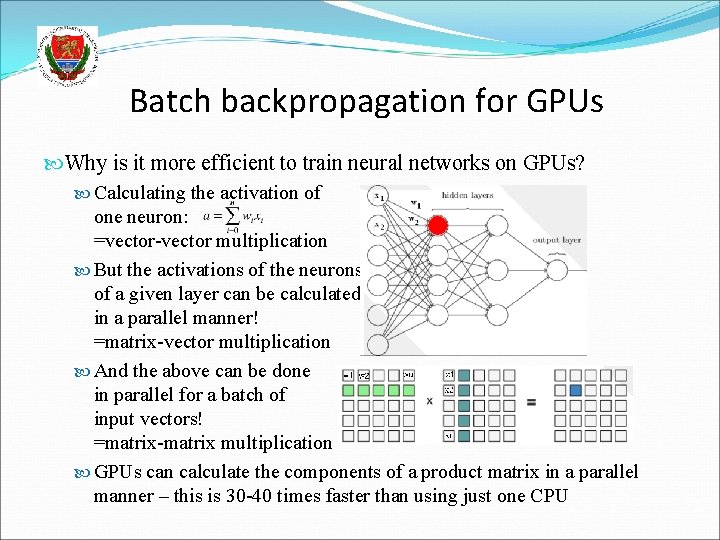
Batch backpropagation for GPUs Why is it more efficient to train neural networks on GPUs? Calculating the activation of one neuron: =vector-vector multiplication But the activations of the neurons of a given layer can be calculated in a parallel manner! =matrix-vector multiplication And the above can be done in parallel for a batch of input vectors! =matrix-matrix multiplication GPUs can calculate the components of a product matrix in a parallel manner – this is 30 -40 times faster than using just one CPU