Artificial Intelligence Uncertainty Chapter 13 Uncertainty What shall

Artificial Intelligence Uncertainty Chapter 13

Uncertainty What shall an agent do when not all is crystal clear? Different types of uncertainty effecting an agent: The state of the world? The effect of actions? Uncertain knowledge of the world: Inputs missing Limited precision in the sensors Incorrect model: action state due to the complexity A changing world

Uncertainty Let action At = leave for airport t minutes before flight Will At get me there on time? Problems: 1) partial observability (road state, other drivers' plans, etc. ) 2) noisy sensors (traffic reports) 3) uncertainty in action outcomes (flat tire, etc. ) 4) immense complexity of modeling and predicting traffic (A 1440 might reasonably be said to get me there on time but I'd have to stay overnight in the airport. . . )

Rational Decisions A rational decision must consider: – The relative importance of the sub-goals – Utility theory – The degree of belief that the sub-goals will be achieved – Probability theory Decision theory = probability theory + utility theory : the agent is rational if and only if it chooses the action that yields the highest expected utility, averaged over all possible outcomes of the action”

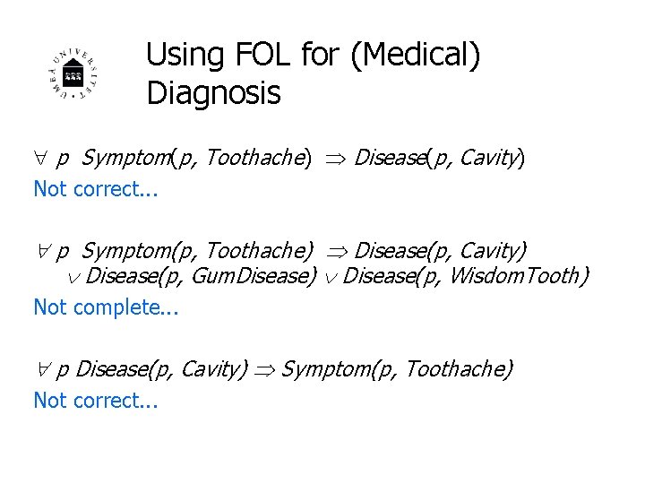
Using FOL for (Medical) Diagnosis p Symptom(p, Toothache) Disease(p, Cavity) Not correct. . . p Symptom(p, Toothache) Disease(p, Cavity) Disease(p, Gum. Disease) Disease(p, Wisdom. Tooth) Not complete. . . p Disease(p, Cavity) Symptom(p, Toothache) Not correct. . .

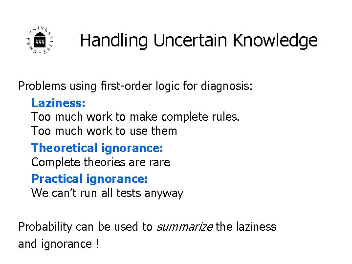
Handling Uncertain Knowledge Problems using first-order logic for diagnosis: Laziness: Too much work to make complete rules. Too much work to use them Theoretical ignorance: Complete theories are rare Practical ignorance: We can’t run all tests anyway Probability can be used to summarize the laziness and ignorance !

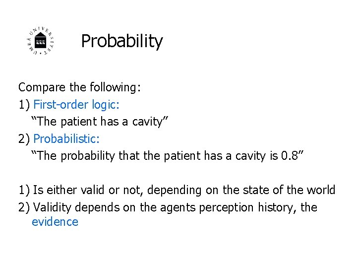
Probability Compare the following: 1) First-order logic: “The patient has a cavity” 2) Probabilistic: “The probability that the patient has a cavity is 0. 8” 1) Is either valid or not, depending on the state of the world 2) Validity depends on the agents perception history, the evidence

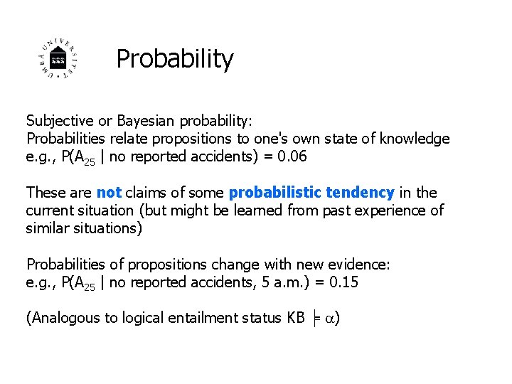
Probability Subjective or Bayesian probability: Probabilities relate propositions to one's own state of knowledge e. g. , P(A 25 | no reported accidents) = 0. 06 These are not claims of some probabilistic tendency in the current situation (but might be learned from past experience of similar situations) Probabilities of propositions change with new evidence: e. g. , P(A 25 | no reported accidents, 5 a. m. ) = 0. 15 (Analogous to logical entailment status KB ╞ )

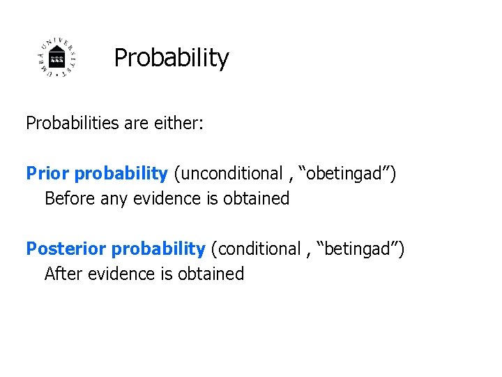
Probability Probabilities are either: Prior probability (unconditional , “obetingad”) Before any evidence is obtained Posterior probability (conditional , “betingad”) After evidence is obtained

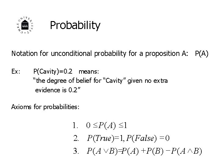
Probability Notation for unconditional probability for a proposition A: P(A) Ex: P(Cavity)=0. 2 means: “the degree of belief for “Cavity” given no extra evidence is 0. 2” Axioms for probabilities: 1. 0 P( A) 1 2. P(True) =1, P( False) = 0 3. P( A Ú B) =P( A) + P( B) - P( A B)

Probability The axioms of probability constrain the possible assignments of probabilities to propositions. An agent that violates the axioms will behave irrationally in some circumstances

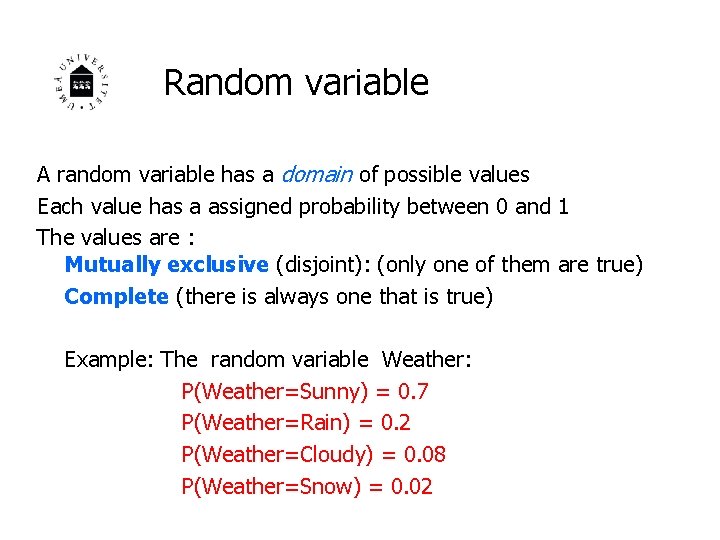
Random variable A random variable has a domain of possible values Each value has a assigned probability between 0 and 1 The values are : Mutually exclusive (disjoint): (only one of them are true) Complete (there is always one that is true) Example: The random variable Weather: P(Weather=Sunny) = 0. 7 P(Weather=Rain) = 0. 2 P(Weather=Cloudy) = 0. 08 P(Weather=Snow) = 0. 02

Random Variable The random variable Weather as a whole is said to have a probability distribution which is a vector (in the discrete case): P(Weather) = [0. 7 0. 2 0. 08 0. 02] (Notice the bold P which is used to denote the prob. distribution)

Random variable - Example - The random variable Season: P(Season = Spring) = 0. 26 or shorter: P(Spring)=0. 26 P(Season = Summer) = 0. 20 P(Season = Autumn) = 0. 28 P(Season = Winter) = 0. 26 The random variable Season has a domain <Spring, Summer, Autumn, Winter> and a probability distribution: P(Season) = [0. 26 0. 20 0. 38 0. 26] The values in the domain are : Mutually exclusive (disjoint): (only one of them are true) Complete (there is always one that is true)

Probability Model Begin with a set - the sample space e. g. , 6 possible rolls of a die. is a sample point/possible world/atomic event A probability space or probability model is a sample space with an assignment P( ) for every 0 P( ) 1 Σ P ( ) = 1 e. g. , P(1) P(2) P(3) P(4) P(5) P(6) 1/6. An event A is any subset of P(A) = Σ{ A} P( ) E. g. , P(die roll < 4) = 1/6 + 1/6 = 1/2

The Joint Probability Distribution Assume that an agent describing the world using the random variables X 1, X 2, . . Xn. The joint probability distribution (or ”joint”) assigns values for all combinations of values on X 1, X 2, . . Xn. Notation: P(X 1, X 2, . . Xn) (i. e. P bold)

The Joint Probability Distribution Joint probability distribution for a set of r. v. s gives the probability of every atomic event on those r. v. s (i. e. , every sample point) P(Weather, Cavity) = a 4 x 2 matrix of values: Weather = sunny rain cloudy snow Cavity = true 0. 144 0. 02 0. 016 0. 02 Cavity = false 0. 576 0. 08 0. 064 0. 08 Every question about a domain can be answered by the joint distribution because every event is a sum of sample points

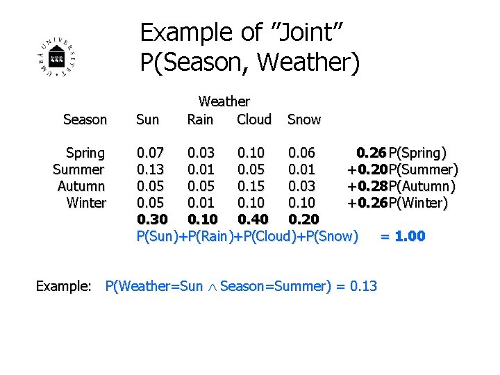
Example of ”Joint” P(Season, Weather) Season Spring Summer Autumn Winter Sun Weather Rain Cloud Snow 0. 07 0. 03 0. 10 0. 06 0. 26 P(Spring) 0. 13 0. 01 0. 05 0. 01 +0. 20 P(Summer) 0. 05 0. 15 0. 03 +0. 28 P(Autumn) 0. 05 0. 01 0. 10 +0. 26 P(Winter) 0. 30 0. 10 0. 40 0. 20 P(Sun)+P(Rain)+P(Cloud)+P(Snow) = 1. 00 Example: P(Weather=Sun Season=Summer) = 0. 13

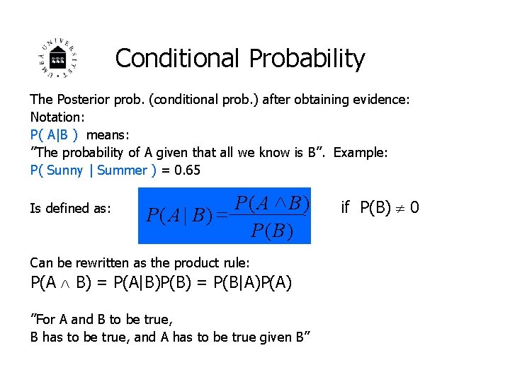
Conditional Probability The Posterior prob. (conditional prob. ) after obtaining evidence: Notation: P( A|B ) means: ”The probability of A given that all we know is B”. Example: P( Sunny | Summer ) = 0. 65 Is defined as: P( A B) P( A | B) = P( B) Can be rewritten as the product rule: P(A B) = P(A|B)P(B) = P(B|A)P(A) ”For A and B to be true, B has to be true, and A has to be true given B” if P(B) 0

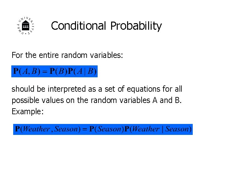
Conditional Probability For the entire random variables: should be interpreted as a set of equations for all possible values on the random variables A and B. Example:

Conditional Probability A general version holds for whole distributions, e. g. , P(Weather, Cavity) = P(Weather|Cavity) P(Cavity) (View as a 4 x 2 set of equations) Chain rule is derived by successive application of product rule: P(X 1, . . . , Xn) = P(X 1, . . . , Xn-1) P(Xn | X 1, . . . , Xn-1) = P(X 1, . . . , Xn-2)P(Xn-1 | X 1, . . . , Xn-2) P(Xn | X 1, . . . , Xn-1) =. . . = ni=1 P(Xi | X 1, . . . , Xi-1)

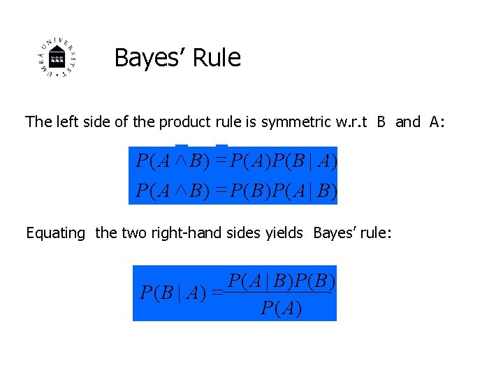
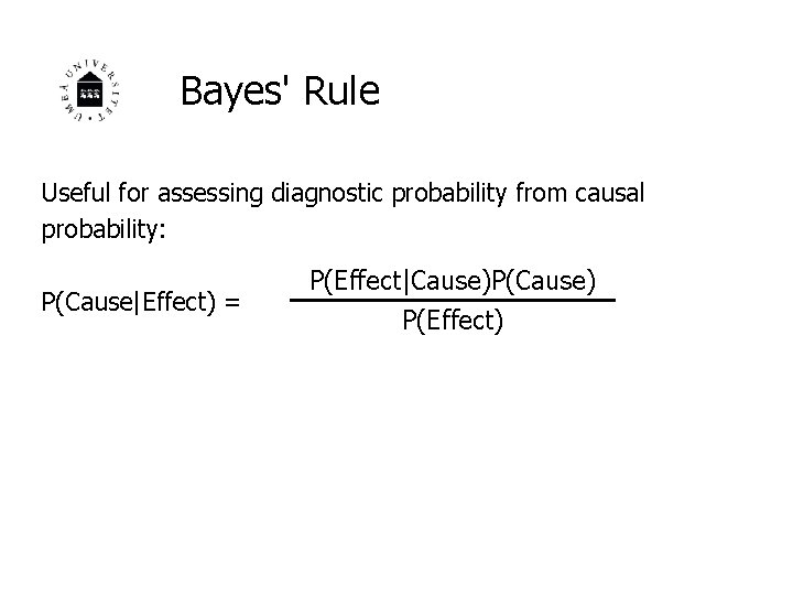
Bayes’ Rule The left side of the product rule is symmetric w. r. t B and A: P( A B) = P( A) P ( B | A) P( A B) = P( B) P( A | B) Equating the two right-hand sides yields Bayes’ rule: P( A | B) P( B) P ( B | A) = P ( A)

Bayes' Rule Useful for assessing diagnostic probability from causal probability: P(Cause|Effect) = P(Effect|Cause)P(Cause) P(Effect)

Example of Medical Diagnosis using Bayes’ rule Known facts: Meningitis causes stiff neck 50% of the time. The probability of a patient having meningitis (M) is 1/50. 000. The probability of a patient having stiff neck (S) is 1/20. Question: What is the probability of meningitis given stiff neck ? Solution: P(S|M)=0. 5 P(M) = 1/50. 000 Note: posterior probability of P(S) = 1/20 meningitis still very small!!

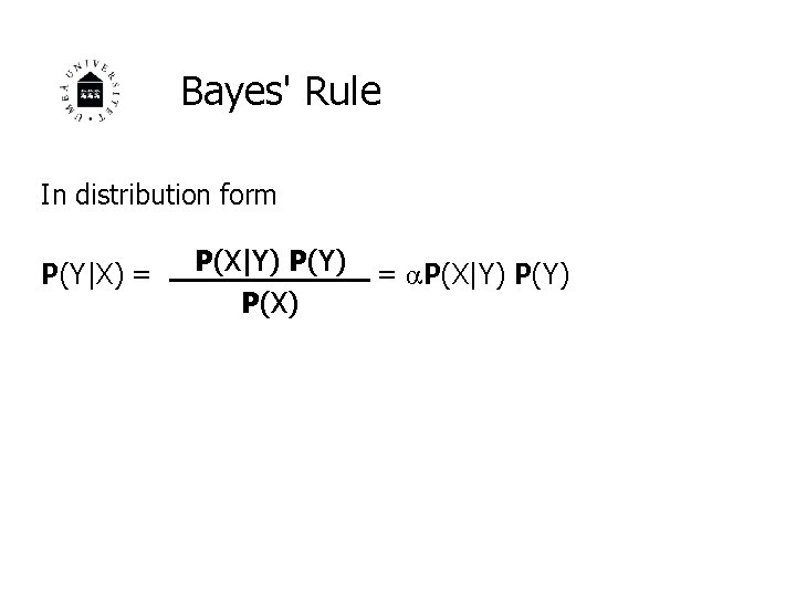
Bayes' Rule In distribution form P(Y|X) = P(X|Y) P(Y) = P(X|Y) P(X)

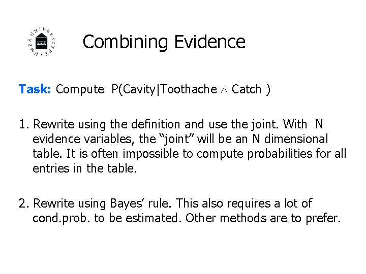
Combining Evidence Task: Compute P(Cavity|Toothache Catch ) 1. Rewrite using the definition and use the joint. With N evidence variables, the “joint” will be an N dimensional table. It is often impossible to compute probabilities for all entries in the table. 2. Rewrite using Bayes’ rule. This also requires a lot of cond. prob. to be estimated. Other methods are to prefer.

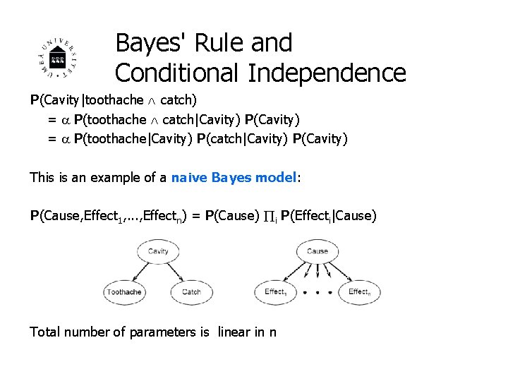
Bayes' Rule and Conditional Independence P(Cavity|toothache catch) = P(toothache catch|Cavity) P(Cavity) = P(toothache|Cavity) P(catch|Cavity) P(Cavity) This is an example of a naive Bayes model: P(Cause, Effect 1, . . . , Effectn) = P(Cause) i P(Effecti|Cause) Total number of parameters is linear in n

Summary Probability can be used to reason about uncertainty Uncertainty arises because of both laziness and ignorance and it is inescapable in complex, dynamic, or inaccessible worlds. Probabilities summarize the agent's beliefs.

Summary Basic probability statements include prior probabilities and conditional probabilities over simple and complex propositions The full joint probability distribution specifies the probability of each complete as assignment of values to random variables. It is usually too large to create or use in its explicit form The axioms of probability constrain the possible assignments of probabilities to propositions. An agent that violates the axioms will behave irrationally in some circumstances

Summary Bayes' rule allows unknown probabilities to be computed from known conditional probabilities, usually in the causal direction. With many pieces of evidence it will in general run into the same scaling problems as does the full joint distribution Conditional independence brought about by direct causal relationships in the domain might allow the full joint distribution to be factored into smaller, conditional distributions The naive Bayes model assumes the conditional independence of all effect variables, given a single cause variable, and grows linearly with the number of effects

Next! Bayesian Network! Chapter 14

Artificial Intelligence Bayesian Network Chapter 14

Introduction Most application requires a way of handling uncertainty to be able to make adequate decisions Bayesian decision theory is a fundamental statistical approach to the problem of complex decision making The expert system developed in the middle of the 1970 s used probabilistic techniques Promising results - but not sufficient because of the exponential number of probabilities required in the full joint distribution

Bayesian Network - Syntax A Bayesian network (or belief network) holds certain properties: 1. A set of random variables U={A 1, …, An}, where each variable has a finite set of mutually exclusive states: Aj={a 1, …, am} 2. A set of directed links or arrow connects pairs of nodes {A 1 A n} 3. Each node has a conditional probability table (CPT) that quantifies the effect that the parents have on the node 4. The graph is a directed acyclic graph (DAG)

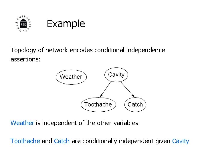
Example Topology of network encodes conditional independence assertions: Weather is independent of the other variables Toothache and Catch are conditionally independent given Cavity

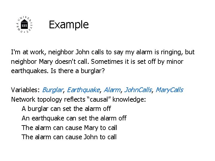
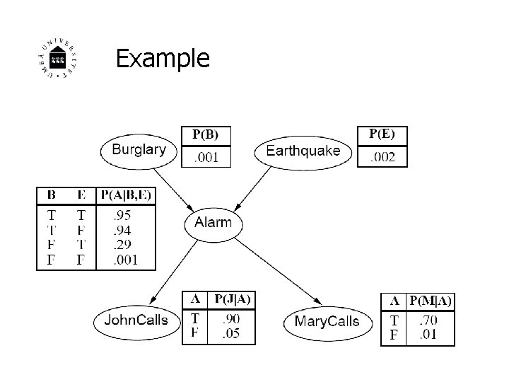
Example I'm at work, neighbor John calls to say my alarm is ringing, but neighbor Mary doesn't call. Sometimes it is set off by minor earthquakes. Is there a burglar? Variables: Burglar, Earthquake, Alarm, John. Calls, Mary. Calls Network topology reflects “causal” knowledge: A burglar can set the alarm off An earthquake can set the alarm off The alarm can cause Mary to call The alarm can cause John to call

Example

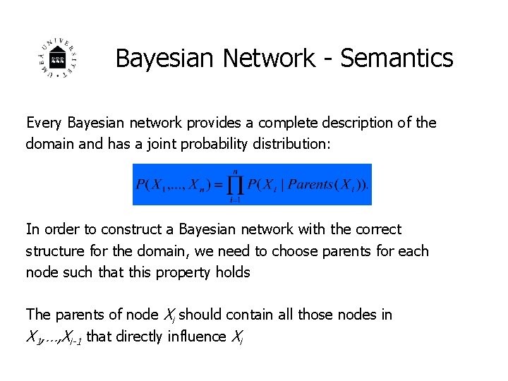
Bayesian Network - Semantics Every Bayesian network provides a complete description of the domain and has a joint probability distribution: In order to construct a Bayesian network with the correct structure for the domain, we need to choose parents for each node such that this property holds The parents of node Xi should contain all those nodes in X 1, …, Xi-1 that directly influence Xi

Example - Semantics "Global" semantics defines the full joint distribution as the product of the local conditional distributions: e. g. , P(j m a b e) = P(j|a) P(m|a) P(a| b, e) P( b) P( e)

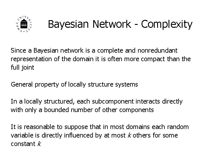
Bayesian Network - Complexity Since a Bayesian network is a complete and nonredundant representation of the domain it is often more compact than the full joint General property of locally structure systems In a locally structured, each subcomponent interacts directly with only a bounded number of other components It is reasonable to suppose that in most domains each random variable is directly influenced by at most k others for some constant k

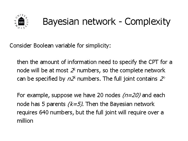
Bayesian network - Complexity Consider Boolean variable for simplicity: then the amount of information need to specify the CPT for a node will be at most 2 k numbers, so the complete network can be specified by n 2 k numbers. The full joint contains 2 n For example, suppose we have 20 nodes (n=20) and each node has 5 parents (k=5). Then the Bayesian network requires 640 numbers, but the full joint will require over a million

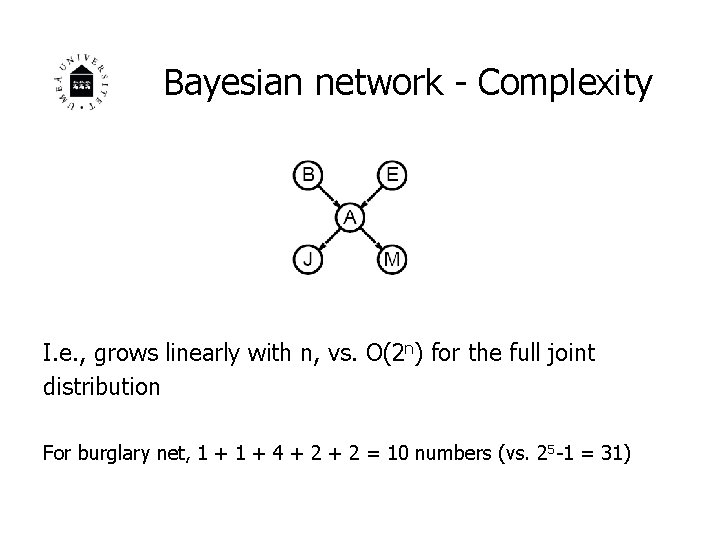
Bayesian network - Complexity I. e. , grows linearly with n, vs. O(2 n) for the full joint distribution For burglary net, 1 + 4 + 2 = 10 numbers (vs. 2 5 -1 = 31)

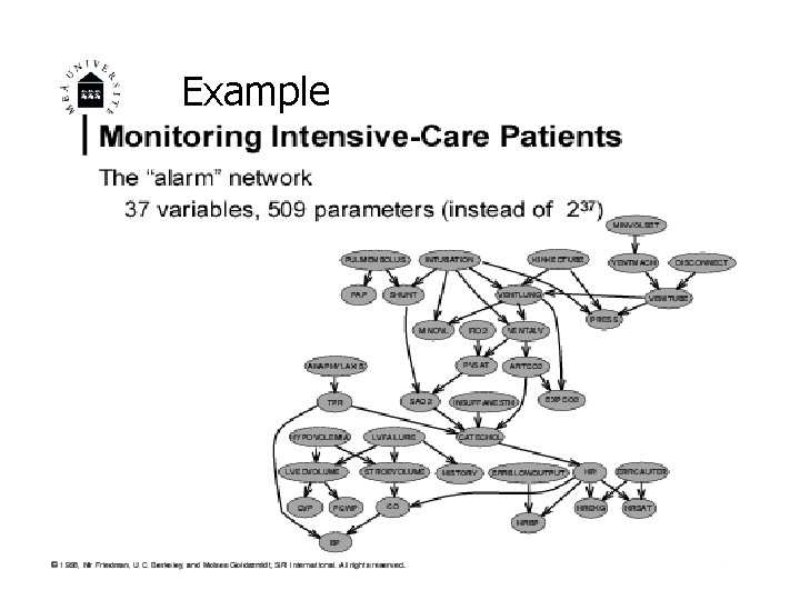
Example

Conditional Independence It is important to be aware of that the links between the variables represent a direct causal relationship New information can be “transmitted” trough nodes in the same and opposite directions of the links This effects the properties of conditional dependency and independency in Bayesian belief networks

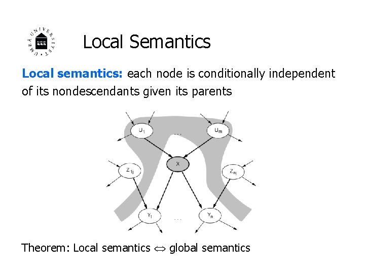
Local Semantics Local semantics: each node is conditionally independent of its nondescendants given its parents Theorem: Local semantics global semantics

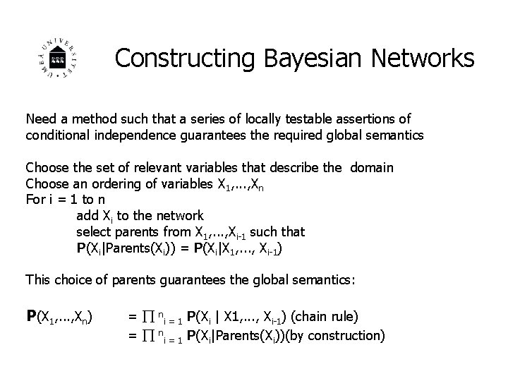
Constructing Bayesian Networks Need a method such that a series of locally testable assertions of conditional independence guarantees the required global semantics Choose the set of relevant variables that describe the domain Choose an ordering of variables X 1, . . . , Xn For i = 1 to n add Xi to the network select parents from X 1, . . . , Xi-1 such that P(Xi|Parents(Xi)) = P(Xi|X 1, . . . , Xi-1) This choice of parents guarantees the global semantics: P(X 1, . . . , Xn) = ni = 1 P(Xi | X 1, . . . , Xi-1) (chain rule) = ni = 1 P(Xi|Parents(Xi))(by construction)

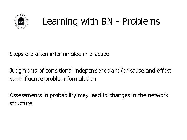
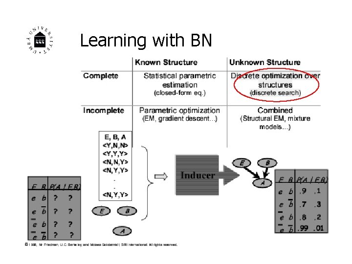
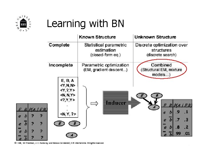
Learning with BN - Problems Steps are often intermingled in practice Judgments of conditional independence and/or cause and effect can influence problem formulation Assessments in probability may lead to changes in the network structure

Learning with BN

Learning with BN

Learning with BN

Learning with BN

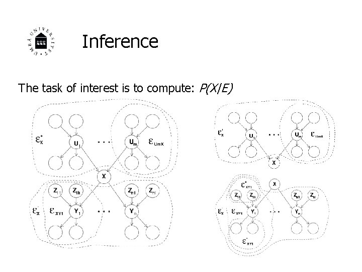
Inference The basic task for any probabilistic inference system is to compute the posterior probability distribution for a set of query variables, given exact values for some evidence variables Bayesian network are flexible enough so that any node can serve as either a query or an evidence variable By adding the evidence we get the posterior probability distribution our query variable will give

Inference The task of interest is to compute: P(X|E)

Summary Bayesian networks, a well-developed representation for uncertain knowledge A Bayesian network is a directed acyclic graph whose nodes correspond to random variables; each node has a conditional distribution for the node, given its parents Bayesian networks provide a concise way to represent conditional independence relationships in the domain

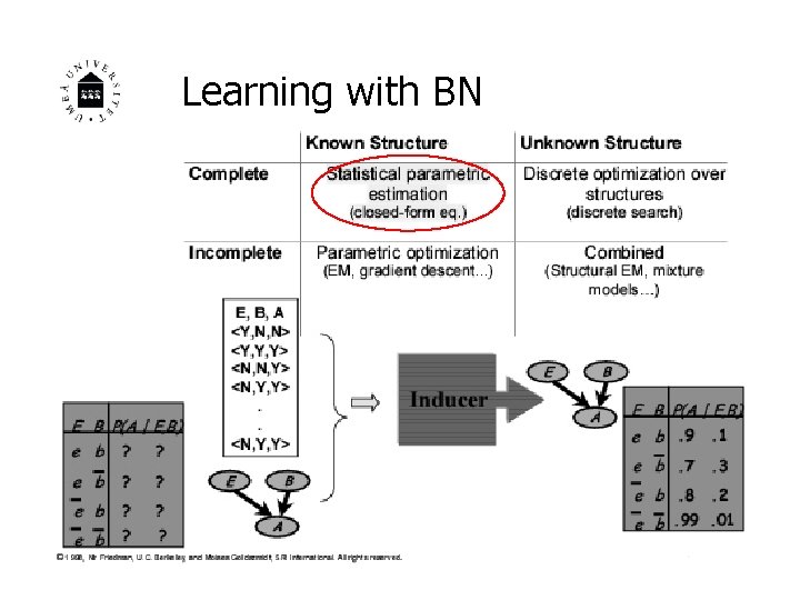
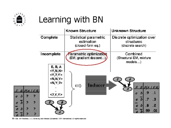
Summary A Bayesian network specifies a full joint distribution; Each joint entry is defined as the product of the corresponding entries in the local conditional distributions A Bayesian network is often exponentially smaller than the full joint distribution Learning in Bayesian networks involves: Parametric estimation, parametric optimization, learning structures, parametric optimization combined with learning structures

Next Time! Repetition!